From Words to Vectors: What Happens in Between?

We use AI tools everyday for various tasks like asking a question about something or solving a problem, and we get responses in seconds.

Now have you ever wondered about how the machine can understand our language and respond to our questions? Or, put another way, how the machine is processing the language and generating a response?

As people who are curious about learning the latest technologies in AI and ML, it’s natural to wonder what is happening internally.

We already have an idea about machine learning models, and one thing we know is that these models work with numbers, or numerical representations of the data, as we preprocess the data and feed it into the model and the model learns patterns in that data.

When i started exploring this, i came across concepts like tokenization, embeddings, transformer architecture, etc. But i don’t want to jump into these concepts directly; instead, let’s build from the basics so that it can be easy to understand the more advanced concepts.

Now the question in front of us is to know how the text is converted to numbers.

One of the classic approaches for doing this is TF-IDF vectorization.

···

You might already know about this concept or you may have even used it in one of your projects.

So why do i start here?

Here, i am building towards embeddings and other important concepts in NLP and AI. Instead of directly starting from concepts like embeddings, i want to start with basics and see how we represent text as numbers, one step at a time.

TF-IDF is a classic topic and i want to explore it in my way by starting with a simple datset and looking at the math and geometry and see what the results actually represent.

If you’re already familiar with TF-IDF, you can use this article as a quick refresher or skip ahead to the upcoming embeddings articles if that’s what you’re curious about.

But if you’re new to text representation, let’s start from the beginning and see what happens when words become numbers.

···

···

What Is TF-IDF?

It’s time to learn what TF-IDF actually is and what it does.

TF-IDF stands for Term Frequency–Inverse Document Frequency.

It combines two ideas.

One is Term Frequency, which means ‘How often does a word appear in a particular document’ and the second is Inverse Document Frequency which means ‘How common or rare is that word across all documents?’

After calculating TF and IDF, we multiply them.

TF-IDF=TF×IDF​.

Let’s see how we calculate this in detail.

···

Let’s Start With a Simple Dataset

For that let’s consider a simple dataset.

We may have any goal with this dataset, like performing classification, finding similar documents, or information retrieval, but we first need to represent these in a numerical form so that a machine learning model can process further.

Step 1: Tokenization

The first step we need to do is to break each review into individual words.

This is called tokenization.

We do this because TF-IDF works by looking at individual terms and how important they are within each document and across all the documents.

D1 : [“the”, “food”, “was”, “good”, “and”, “fresh”]

D2 : [“the”, “food”, “was”, “good”, “and”, “tasty”]

D3 : [“the”, “food”, “was”, “bad”, “and”, “stale”]

D4 : [“the”, “food”, “was”, “bad”, “and”, “tasteless”]

This is what we get after tokenization, and each word is called token.

···

Step 2: Building the Vocabulary

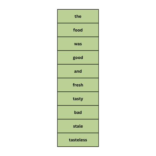
The next step is to create a vocabulary which is the collection of all the unique values across all the documents we have in the dataset.

For our data, the vocabulary we have is:

···

Step 3: Term Frequency (TF)

Now we calculate the term frequency or simply we call it as TF.

This is the first part of TF-IDF.

We calculate the term frequency using:

Here, ‘t’ represents a term(word) and ‘d’ represents the document(review).

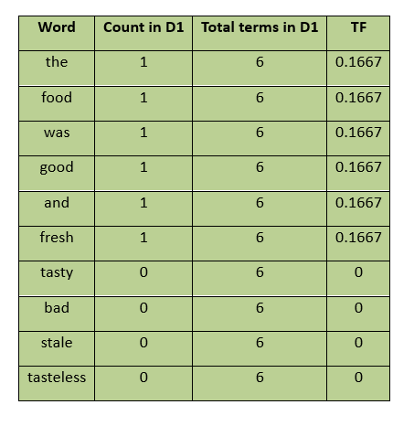
Now let’s consider D1, after tokenization we have: [“the”, “food”, “was”, “good”, “and”, “fresh”].

Consider the word ‘food’, which appears only once in the document.

Therefore, the term frequency of ‘food’ is 1/6.

Every word appears only once in D1, which means the term frequency here is same for all the words.

Now if we look at our vocabulary, it contains all the unique words from all four documents, not just the words in D1.

So, when we create the numerical representation for D1, we need to have a value for every word in this vocabulary.

For example, consider the word ‘tasty’, it doesn’t appear in D1.

The TF of ‘tasty’ in D1 is zero.

The same thing will be applied to the other words which are not in D1.

So, in the order of our vocabulary, the TF values of D1 are:

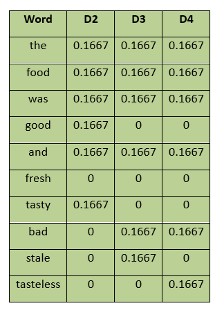
In the same way, we get TF values for all the words across all documents.

···

Now we have calculated the Term Frequency for all the four documents.

We observed that the TF value depends only on how often a word appears within a particular document.

But TF alone is not enough.

For example, consider the words ‘the’ and ‘fresh’ in D1.

Both words appear only once in D1, but ‘the’ appears in all the four documents.

What we can observe here?

We can say that TF alone cannot tell us that the word ‘fresh’ is more informative for distinguishing D1 from the other documents.

So, we need another measure that considers all the documents.

This brings us to IDF which is Inverse Document Frequency.

···

Step 4: Document Frequency (DF)

Before proceeding with IDF, let’s first understand the Document Frequency.

Document Frequency tells us in how many documents the particular word appears.

We must observe that we are counting documents, not the total number of times a word appears.

For example, consider ‘the’: It appears in all the four documents.

Therefore, the document frequency for ‘the’ is:

We can find this for every word in the vocabulary.

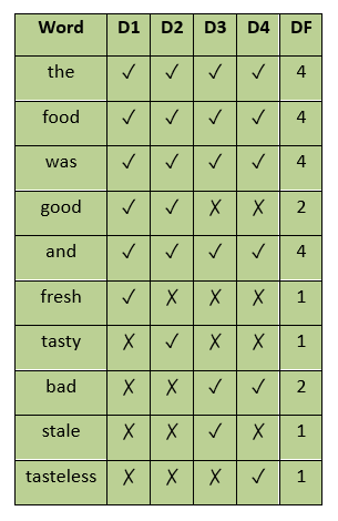
Now we have the DF for every word in our vocabulary. But what can we do with it?

If we observe the DF values, we can see that some words have a high DF, while others have a low DF.

We can sense that words with a low DF can be more significant when distinguishing a particular document from the others.

So, we need a measure that gives higher weight to words with low DF and lower weight to words with high DF.

This is where the Inverse Document Frequency(IDF) comes in.

Here, we are using IDF because we want the weight of the word to move in opposite direction to DF, which means higher DF gives lower weight, while lower DF gives higher weight.

···

Step 5: Inverse Document Frequency (IDF)

Now it’s time to calculate the IDF values for our vocabulary.

The formula we use is:

Here:

N is the total number of documents, and DF(t) is the number of documents containing the term t.

Here, we use the logarithm to compress the range of IDF values, so that very rare words do not receive disproportionately large weights.

In our dataset, we have four documents.

Now we again consider the word ‘the’:

From the Document Frequency table, we have:

Substituting the values into formula, we get:

The IDF value for ‘the’ is 0.

Now, let’s consider another word ‘good’, we get:

We can observe that the IDF value of ‘good’ is higher than ‘the’, because ‘good’ appears in fewer documents.

Using the same process, we can calculate the IDF values for every word in the vocabulary.

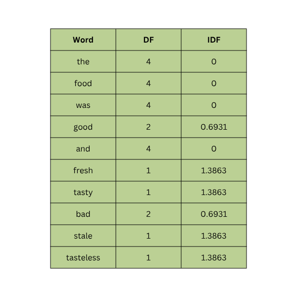
From the above table, we can observe that:

The words ‘the’, ‘food’, ‘was’ and ‘and’ appear in all four documents, so their IDF is 0.

The words ‘good’ and ‘bad’ appear in two documents, so their IDF is approximately 0.6931.

The words ‘fresh’, ‘tasty’, ‘stale’ and ‘tasteless’ appear in only one document, so they have the highest IDF value in our dataset, approximately 1.3863.

At this point, we have both pieces we need:

One is TF which tells us how frequently a word appears in a particular document and

the second is IDF which tells us how common or rare that word is across the collection of documents.

···

Step 6: Calculating TF-IDF

The next step is to combine these two values to obtain the actual TF-IDF score for each word. We do this by multiplying TF and IDF.

Now, let’s consider our first document D1:

‘The food was good and fresh’

From the earlier calculations, we have

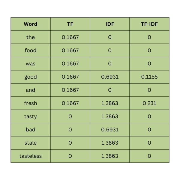
TF(the,D1)=0.1667 and IDF(the)=0.

Therefore:

The TF-IDF score for ‘the’ is zero, this happened because it appears in every document. It’s TF tells us it appears in D1 but it’s IDF tells us that it is common across all documents.

Let’s apply the same idea to ‘good’.

We already know:

TF(good,D1)=0.1667 and IDF(good)=0.6931

This way we calculate the TF-IDF scores for all the words in D1.

···

From TF-IDF Scores to Vectors

We now have the TF-IDF scores for every word in D1.

The order of our vocabulary is:

[the, food, was, good, and, fresh, tasty, bad, stale, tasteless]

Now, we can write the TF-IDF representation of D1 as:

First we have the review D1 as text, but now we represented it using numbers.

We can observe that the numbers are in a fixed order, with each number representing a word from our vocabulary.

The first number represents the, the second represents food, the fourth represents good, and so on.

As it has ordered collection of numerical values, we can represent it as a vector.

In our vocabulary, we have 10 words, so here we have a 10-dimensional vector, where each dimensions corresponds to one word in the vocabulary.

In the same way, we get the TF-IDF representations for the other documents.

We now have an idea of the math behind TF-IDF.

···

Implementing TF-IDF in Python

But in real-world applications, we use Python and libraries such as scikit-learn to calculate the values.

Let’s have a look at how it is implemented in python.

Code:

from sklearn.feature_extraction.text import TfidfVectorizer# Our reviewsreviews = [    "The food was good and fresh",    "The food was good and tasty",    "The food was bad and stale",    "The food was bad and tasteless"]# Create the TF-IDF vectorizervectorizer = TfidfVectorizer()# Convert the reviews into TF-IDF vectorsX = vectorizer.fit_transform(reviews)# Get the vocabulary/featuresprint("Vocabulary:")print(vectorizer.get_feature_names_out())# Display the TF-IDF matrixprint("nTF-IDF Matrix:")print(X.toarray())# Display the shape of the matrixprint("nShape:")print(X.shape)

Output:

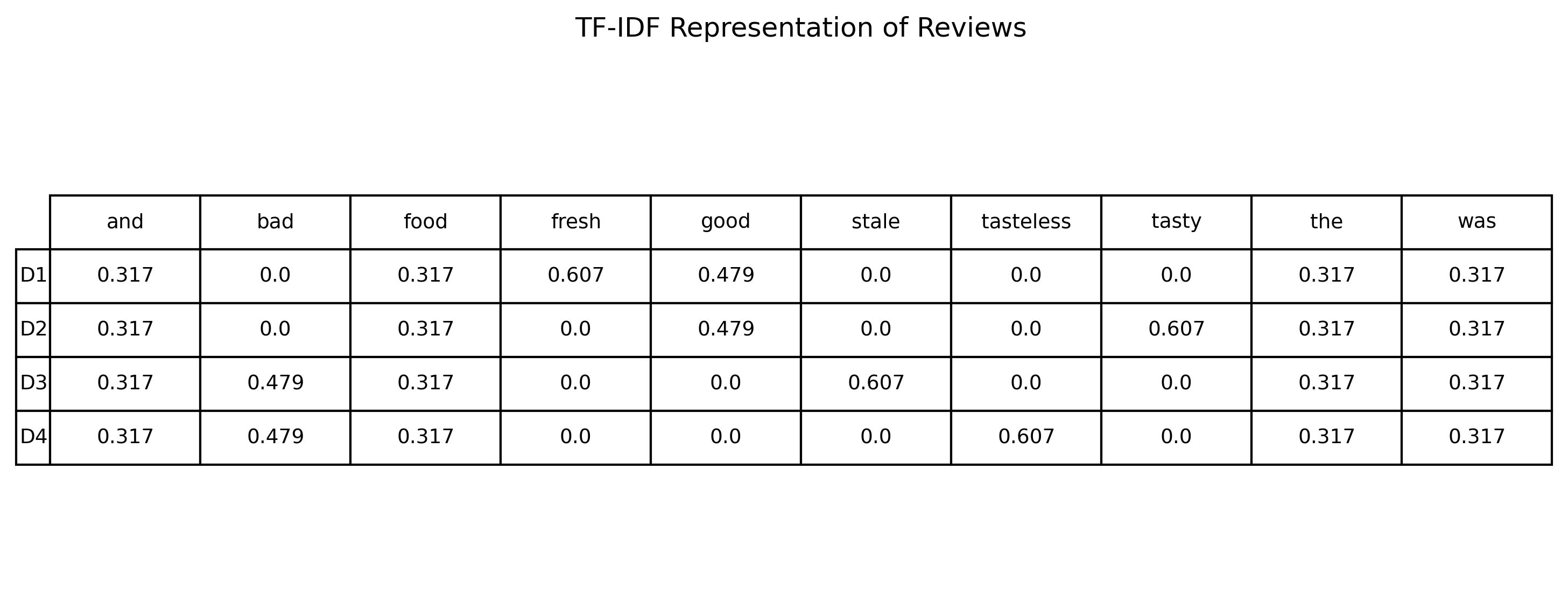
Why Are the Python Values Different?

We can observe that the values we got by using python are different from what we got by manual calculation.

This happens because TF-IDF uses a smoothed IDF formula.

The other thing is that TF-IDF vectorizer also normalizes each document vector, which results in scaling the values in a vector based on the overall length of that vector.

But why this is done in python implementation.

It is because smoothing is used to change the behavior of IDF at boundary cases, for example consider word ‘the’ in our vocabulary, it’s IDF value is 0 but when we use the smoothed formula it becomes 1.

The python implementations such as scikit-learn use these methods to keep the IDF calculation in a consistent form.

While normalization reduces the influence of document length on the magnitude of the TF-IDF vector.

For example, a longer document will produce a larger-magnitude vector simply because it contains more words. Normalization scales the vector, allowing us to focus more on the pattern of TF-IDF values rather than the overall size of the vector.

···

Visualizing TF-IDF Vectors With PCA

Now we have four 10-dimensional vectors.

We want to visualize them, but we cannot directly plot a 10-dimensional vector space on a 2D graph.

What we can do is, use a dimensionality reduction technique to reduce the number of dimensions and visualize the resulting representations in a 2D plot.

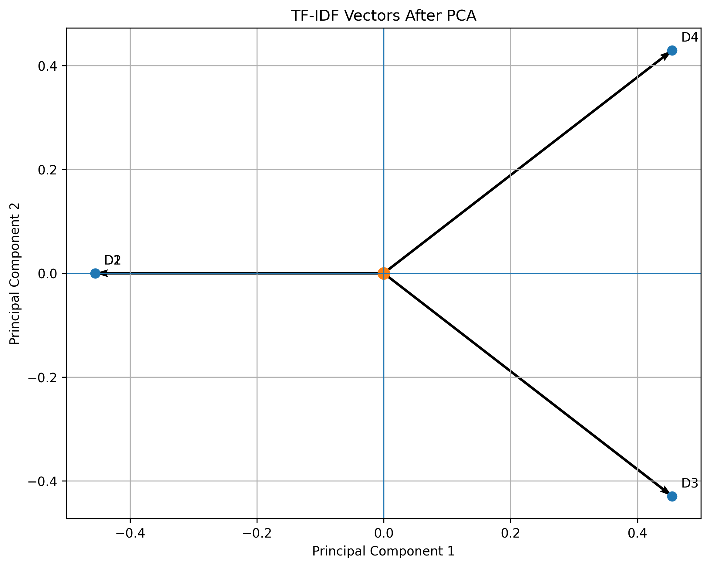
Before applying PCA, each review was represented by 10 TF-IDF values and after applying PCA, each review is represented by just two values, which we can call as a 2d-vector.

In this 2D PCA projection, documents with similar numerical representations tend to appear closer together.

We will discuss about every dimensionality reduction technique in detail in the upcoming articles.

···

Using TF-IDF for Text Classification

We now converted our reviews to the numerical representations, but this is not our final goal.

Our final goal is to use this numerical representations to perform a real world task like classification.

If you remember, our dataset has labels ‘1’ and ‘0’.

‘1’ means positive and ‘0’ means negative.

Now we can use these numerical representations as our input features and labels as the target for a machine learning model.

For example, let’s use the logistic regression for classification.

For classification, we will use the TF-IDF representation from our Python implementation, not the 2D representation produced by PCA.

First, let’s see how our dataset now looks:

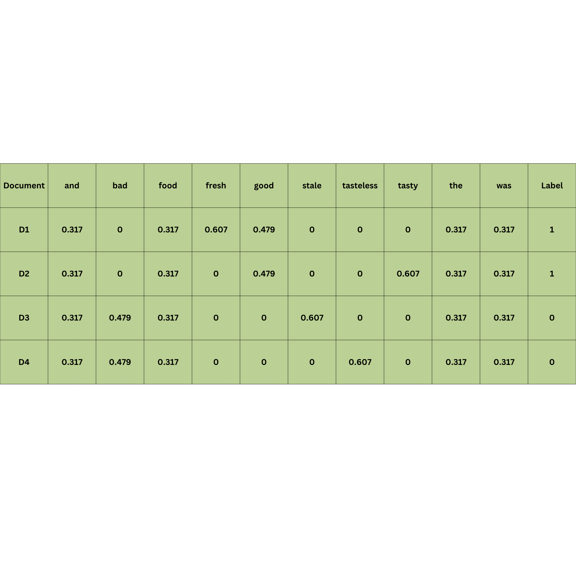
Our dataset is no longer made up of text. We have transformed it into a numerical machine learning dataset. Each word in the vocabulary is a feature.

Now let’s use Python to implement the logistic regression to predict the label.

We all know that logistic regression learns a weight for each feature and also learns a bias.

The model first calculates a score:

Later we use the sigmoid function to get the value that can be interpreted as a probability between 0 and 1.

Now let’s look at the code.

from sklearn.feature_extraction.text import TfidfVectorizerfrom sklearn.linear_model import LogisticRegression# Our datasetreviews = [    "The food was good and fresh",    "The food was good and tasty",    "The food was bad and stale",    "The food was bad and tasteless"]# Target Labelslabels = [1, 1, 0, 0]# Convert text into TF-IDF featuresvectorizer = TfidfVectorizer()X = vectorizer.fit_transform(reviews)# Create and train the Logistic Regression modelmodel = LogisticRegression()model.fit(X, labels)# Display the learned weightsfeature_names = vectorizer.get_feature_names_out()print("Learned weights:")for word, weight in zip(feature_names, model.coef_[0]):    print(f"{word}: {weight:.4f}")# Display the learned biasprint("nBias:", model.intercept_[0])# Predict the training examplespredictions = model.predict(X)print("nPredictions:", predictions)# Predict for a new reviewnew_review = ["The food was fresh"]new_vector = vectorizer.transform(new_review)print("nPrediction probability:")print(model.predict_proba(new_vector))print("nPredicted class:")print(model.predict(new_vector))

Output:

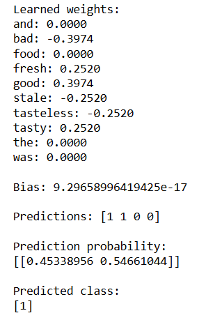
We have now trained the Logistic Regression model and used it to predict the label for a new review.

Here, we can observe that the words in the new review are already present in our vocabulary. We then converted the new review into a TF-IDF vector using the same fitted vectorizer that we used for the training data.

···

What Happens When We Encounter a New Word?

For example, we have a new review: ‘the food was delicious’.

The word ‘delicious’ is not present in our vocabulary. The model has no learned feature or weight for “delicious.”

Let’s predict the label for this review.

Code:

new_review = ["The food was delicious"]new_vector = vectorizer.transform(new_review)print("TF-IDF vector:")print(new_vector.toarray())print("Prediction:")print(model.predict(new_vector))print("Prediction probability:")print(model.predict_proba(new_vector))

Output:

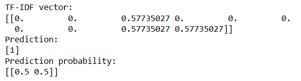
From the output, we can observe something interesting. As the word ‘delicious’ is not in vocabulary, it does not contribute any feature to the TF-IDF vector. So the model makes its prediction using only the other three words which it knows already.

We can also see that the prediction probability is 50% for each class. This means the model does not have enough information from the available features to clearly distinguish between the two classes for this review.

Let’s see what actually happened with our new review “the food was delicious”.

The fitted vectorizer checks each word against the vocabulary it learned from the training data. It uses the IDF values already learned from the training data.

The words “the,” “food,” and “was” are present in the vocabulary, while “delicious” is not. Therefore, no feature is created for “delicious,” and its contribution to the vector is 0.

The three known words receive TF-IDF values, resulting in approximately 0.577 for each of them. This gives us the vector shown below.

[0. 0. 0.577 0. 0. 0. 0. 0. 0.577 0.577]

···

Limitations of TF-IDF

What we can understand from this?

We can observe a limitation of TF-IDF, where a word that was not present in the training vocabulary cannot contribute to the model’s prediction.

There is also another limitation, even when words are present in vocabulary, it treats them as separate features.

For example, if we have words ‘good’ and ‘excellent’ in our vocabulary, they are represented as two different words, without any inherent understanding that they have similar meanings.

That doesn’t mean we don’t use TF-IDF at all. It is still used in tasks like text classification, spam detection etc.

···

From TF-IDF to Embeddings

Now the question is instead of representing a word simply as a feature with a TF-IDF score, can we represent a word using numbers that capture its relationships with other words?

This is where embeddings come in.

They are widely used in applications such as semantic search, question answering, recommendation systems, retrieval augmented generation (RAG) etc.

···

I hope you found this blog useful for understanding the basics on how text can be converted into a numerical representation.

If you think something is missing or could be improved, feel free to leave a comment on Linkedin.

In the next article, we’ll start from the basics and explore how embeddings represent words as vectors.

By the way, if you haven’t read my recent blog on sigmoid function, you can read it here.

Thanks for reading!