When Labels Say No, But Embeddings Say Yes

“There is nothing more deceptive than an obvious fact.”
— Sherlock Holmes, in “The Boscombe Valley Mystery” by Arthur Conan Doyle

1. Introduction

You just won the lottery, and your first purchase will fulfill a childhood dream: buying a Ferrari. You visit a luxury car website, find a gorgeous Ferrari sports car, and click “Find Similar.” The results? Four Ferraris (great!), one Lamborghini (cool!), and a Ferrari SUV (wait, what?). You love the Ferrari and Lamborghini recommendations. But the Ferrari SUV? That’s way off from what you had in mind.

Why did the Lamborghini appear? Because it shares the visual characteristics that attracted you to the Ferrari: similar low profile, smooth curves, and sporty design. And the Ferrari SUV? Perhaps the retrieval system gave a large weight to characteristics associated with the Ferrari brand, despite its very different shape. Both results reflect similarity, but two very different notions of what it means to be similar.

Now comes the interesting part.

Suppose the search engine is evaluated using a benchmark that considers two cars relevant only if they share the same brand label. The Lamborghini would be counted as a mistake, while the Ferrari SUV would receive full credit.

So the car you love is wrong, and the car you don’t want is right. Something seems a little backward here, doesn’t it?

This example shows a big limitation of category-based retrieval evaluation: semantic similarity and categorical agreement aren’t necessarily the same. A retrieval system may discover meaningful relationships between objects from different categories, but get a penalty just because their labels don’t match.

This raises an intriguing question:

When embeddings find meaningful similarities that labels fail to recognize, should we really call those retrievals mistakes?

In this article, we investigate this question using CLIP (Contrastive Language–Image Pre-training), one of the most well-known vision-language models for representing images and text in a shared embedding space.

Our experiment uses a Kaggle dataset containing 9,315 images across 23 architectural styles. Why architecture? Because buildings from different architectural styles can have similar roofs, windows, materials, symmetry, and decorative details. Two buildings can look very similar without having the same architectural label.

This is a perfect case for investigating whether CLIP is truly confused—or whether our evaluation criteria are sometimes too rigid.

1.1 What We Will Explore

We begin by explaining how CLIP represents images as embeddings and measures similarity using cosine similarity.

Next, we introduce our architectural image dataset and establish CLIP’s baseline retrieval performance using the following: Precision@1, Precision@5, and Precision@10.

Precision@k (P@k) measures the proportion of the top k retrieved images that are relevant to the query. In our experiments, an image is considered relevant if it has the same architectural style label as the query image. For example, a Precision@5 of 0.80 means that four of the five highest-ranked retrieved images belong to the same architectural style as the query.

We then go beyond category labels and measure architectural similarity using roof types, materials, symmetry, windows, and other distinctive features.

We then take a closer look at CLIP’s apparent mistakes, which we call label mismatches. Are these mismatches random, or does CLIP tend to retrieve architecturally related styles? We look at similarity scores, common mismatches, and how architectural styles are related.

Finally, we consider what all this means for retrieval evaluation. Should relevance be a simple yes or no, or can measuring degrees of similarity give us a better picture of retrieval quality?

Our goal is not to prove that CLIP is always right. Some mistakes are just mistakes. But perhaps others deserve a second look.

After all, if you asked for a Ferrari sports car and received a Lamborghini, would you really complain?

2. How CLIP Sees Similarity

Once we have the embeddings, we need a mathematical way to compare them.

One of the most widely used measures is cosine similarity:

Cosine similarity measures the angle between two vectors rather than their absolute lengths. A value of 1 indicates the vectors point in the same direction, while 0 indicates they are orthogonal.

In our retrieval pipeline, we normalize the embeddings and rank candidate images by their cosine similarity to the query embedding. The result is a ranked list of images according to their proximity in CLIP‘s learned representation.

To get a glimpse of this high-dimensional space, we use Principal Component Analysis (PCA) to project CLIP’s 512-dimensional image embeddings onto two dimensions.

The PCA projection of CLIP’s image embeddings shows some clustering by architectural style, but also considerable overlap between different styles. However, the first two principal components explain only 21.3% of the total variance. Therefore, the two-dimensional projection captures only a small portion of the information in the original 512-dimensional embedding space, and the apparent overlap should be interpreted with caution.

So far, so good. But notice something important:

Cosine similarity tells us how close two images are in CLIP’s embedding space. It does not tell us which characteristics produced that similarity—or whether those characteristics are relevant to the user’s search.

CLIP’s embeddings capture information about objects, their appearance, composition, and meaning. However, the model does not tell us how much each of these factors contributes to a similarity score.

This distinction matters because two images can be close in embedding space for reasons that have little to do with the characteristics we actually care about.

2.2 When we get a label mismatch

Consider an image of a Gothic building submitted as a query. Suppose CLIP retrieves another Gothic building as its closest match. Excellent! A label-based benchmark gives it full credit.

Now suppose it retrieves a Romanesque building instead. The benchmark marks the result as incorrect because the architectural labels differ. But Gothic and Romanesque buildings have much in common, including stone construction, arches, heavy structural elements, and historical influences.

Could CLIP have captured a meaningful architectural relationship? Possibly.

Of course, not every label mismatch is a hidden success. Sometimes CLIP may retrieve a building because of its background, lighting, photographic perspective, or other characteristics unrelated to architectural style.

We want to find out whether CLIP’s label mismatches reflect real similarities between architectural styles or just coincidental ones. To do this, we need to go beyond correct and incorrect labels and measure how much architectural styles have in common.

And that brings us to our experiment.

3. From Ferraris to Facades: Our Architectural Experiment

Architectural styles often share characteristics, so we can examine whether CLIP’s label mismatches reflect meaningful similarities rather than arbitrary retrievals.

3.1 The Dataset

We began with a Kaggle architectural image dataset containing 10,113 images representing 25 architectural styles. We excluded two categories—Achaemenid and Ancient Egyptian architecture—because they mainly include ancient monuments, while our search system focuses on houses and similar buildings. After removing these categories, our final dataset contained 9,315 images across 23 architectural styles.

The collection includes Gothic, Romanesque, Bauhaus, International, Georgian, Greek Revival, Art Deco, and other architectural styles. Each image has an architectural-style label, allowing us to evaluate retrieval performance using conventional category-based metrics.

But we want to go further.

When CLIP retrieves an image from a different architectural style, we want to know whether the query and retrieved styles share meaningful architectural characteristics. For that, we need an additional source of information beyond CLIP’s embeddings and the dataset’s labels.

3.2 Two Ways to Judge a Retrieval

We evaluate CLIP from two complementary perspectives.

First: Categorical relevance.

This is the conventional approach. A retrieved image is considered relevant if its architectural-style label matches the query’s label. We calculate Precision@1, Precision@5, and Precision@10 to establish our baseline. These metrics tell us how effectively CLIP retrieves images belonging to the same labeled architectural category.

Second: Architectural similarity.

Here, we look beyond the labels.

We construct a structured representation of architectural characteristics, including roof types, materials, symmetry, window configurations, and distinctive features. Using these characteristics, we calculate a similarity measure between architectural styles.

This gives us an independent way to investigate whether label-mismatched retrievals tend to involve styles that share architectural features. It is important to note that our measure compares architectural styles based on their common features. It does not compare individual buildings. Buildings from related architectural styles may still look very different.

Our objective is not to declare every label mismatch correct, nor to replace conventional retrieval metrics. Instead, we want to examine what those metrics might be missing.

4. The Baseline: How Often Does CLIP Get It Right?

Before questioning whether CLIP’s mistakes are really mistakes, we need to establish how well it performs according to conventional retrieval metrics.

Our experiment uses 9,315 images representing 23 architectural styles. Each image serves as a query, and CLIP retrieves the most similar images from the collection using cosine similarity between their embeddings. The query image itself is excluded from the retrieval results.

For this initial evaluation, we adopt a straightforward definition of relevance: a retrieved image is considered correct if it has the same architectural-style label as the query.

No partial credit. No architectural interpretation. Just matching labels. This is described below in Section 4.1.

4.1 Measuring Retrieval Performance

We evaluate CLIP using three standard metrics: Precision@1, Precision@5, and Precision@10.

Precision@1 measures whether the highest-ranked retrieved image has the same architectural-style label as the query. Precision@5 and Precision@10 measure the proportion of matching-label images among the top five and top ten retrieved results, respectively. Table 1 shows the results.

Metric	Precision
Precision@1	0.7354
Precision@5	0.6461
Precision@10	0.6065

Table 1. CLIP baseline retrieval performance using exact architectural-style label matching.

At first glance, CLIP performs reasonably well. Approximately 73.5% of the highest-ranked retrieved images share the query’s architectural-style label. However, precision decreases as we consider more retrieved images. Among the top five results, approximately 64.6% have matching labels. Among the top ten, that proportion falls to 60.7%.

This decline is not particularly surprising. As we move further down the ranked list, CLIP includes images that are progressively less similar to the query according to its embedding-based similarity measure.

But there is another way to interpret these results.

4.2 The Other 26.5%

About 73.5% of CLIP’s top-ranked retrievals match the query’s architectural style. But what about the remaining 26.5%?

Of our 9,315 queries, 2,465 produced a top-ranked retrieval (Precision@1) with a different style label. All were counted as incorrect, even when the styles were closely related, such as Gothic and Romanesque or Bauhaus and International Style.

The benchmark makes no distinction between retrieving a closely related architectural style and retrieving one with substantially different characteristics. Both receive the same score: zero.

Precision@1 measures how often labels match, but does it tell us everything about retrieval quality? Our next step is to examine the architectural relationships behind CLIP’s label mismatches, using a similarity measure independent of its embeddings.

5. Beyond Style Labels: Measuring Architectural Similarity

To measure these similarities, we developed a feature-based measure, M_feature, that compares architectural styles based on shared characteristics rather than labels.

However, not all architectural characteristics can be compared in the same way. Some, such as roof types and construction materials, can be represented as sets of attributes. Others, such as symmetry and ornamentation, are better represented using ordered levels.

We therefore use two complementary similarity measures—Jaccard similarity and ordinal similarity—and combine them into a single architectural similarity score.

Importantly, this measure is independent of CLIP’s embeddings and retrieval scores.

5.1 Representing Architectural Styles Through Their Features

We considered five groups of features:

• Overall Form: Symmetry, verticality, geometric regularity, massing complexity, and ornamentation.

• Roof Types: Characteristic roof configurations associated with each style.

• Architectural Elements: Distinctive structural and decorative features, such as arches and columns.

• Windows: Characteristic window shapes and arrangements.

• Materials: Common construction materials, including stone, brick, wood, stucco, and glass or steel.

For each of the 23 architectural styles, we created a profile in a predefined dictionary called STYLE_PROFILES. We manually created this dictionary using typical architectural features, assigning ordinal values based on their prominence in each style.

We represented the four feature groups—Roof Types, Architectural Elements, Windows, and Materials—as sets of characteristic attributes. For example, Bauhaus and International Style share several modernist characteristics, including geometric regularity, flat roofs, and large glazed windows. Gothic and Romanesque architecture share features such as steep roofs, arches, towers, and stone construction, despite their important historical and stylistic differences.

The profiles describe the typical characteristics of architectural styles rather than the specific features of individual buildings. This distinction matters. A particular Gothic building may differ substantially from another Gothic building, just as two buildings belonging to different styles may look remarkably similar.

Our objective is not to describe every building perfectly. It is to establish a structured, interpretable representation of architectural relationships.

5.2 Comparing Sets of Architectural Features: Jaccard Similarity

Let’s begin with characteristics that can be represented as sets.

For Roof Types, Architectural Elements, Windows, and Materials, we used Jaccard similarity, which measures how many features two styles share relative to the total number of distinct features associated with either style.

Equation 1. Jaccard similarity

Here, A and B are sets of features associated with two architectural styles. The numerator counts their shared features, while the denominator counts all distinct features present in either style.

Example: Comparing the roof types of Gothic and Romanesque architecture

According to our architectural profiles:

• Gothic roof types: {gable, steep}

• Romanesque roof types: {gable, steep}

The two styles share both roof characteristics. Their intersection contains two features, and their union also contains two features. Therefore:

Equation 2.

The roof similarity is 1.0, indicating complete overlap between the roof characteristics encoded in our profiles.

Let’s consider a less similar pair.

Example: Comparing the materials of Bauhaus and International Style

Our profiles specify:

• Bauhaus: {glass_steel, concrete, stucco}

• International Style: {glass_steel, concrete}

The styles share two materials, while their union contains three distinct materials.

Therefore:

Equation 3.

Their material similarity is approximately 0.667.

Notice that Jaccard similarity does not measure whether two materials are themselves similar. It simply measures the overlap between the sets of attributes we assigned to the styles.

We apply this calculation separately to roof types, architectural elements, windows, and materials. When both feature sets are empty, the component is treated as unavailable rather than assigning similarity based on shared absences.

5.3 Comparing Overall Form: Ordinal Similarity

The features that comprise the Overall Form feature describe degrees rather than the presence or absence of particular attributes. Consider Ornamentation. A building may have minimal, moderate, or elaborate ornamentation. Similarly, architectural Symmetry may range from predominantly asymmetric to highly symmetric. We represented five Overall Form characteristics using ordinal values ranging from 0 to 2:

Characteristic	0	1	2
Symmetry	Low	Moderate	High
Verticality	Low	Moderate	High
Geometric regularity	Low	Moderate	High
Massing complexity	Low	Moderate	High
Ornamentation	Low	Moderate	High

Table 2.

To compare two styles, we calculate how far apart their assigned values are:

Equation 4.

Here, a_k and b_k are the ordinal values assigned to characteristic k for architectural styles A and B.

The calculation produces three possible similarity values:

• Identical ordinal values: similarity = 1.

• A difference of one level: similarity = 0.5.

• A difference of two levels: similarity = 0.

Consider the following example: We want to compare the Overall Form of Gothic and Bauhaus architectures. The Overall Form attributes of these architectures contain the following ordinal values:

Characteristic	Gothic	Bauhaus	Similarity
Symmetry	1	1	1.0
Verticality	2	1	0.5
Geometric regularity	1	2	0.5
Massing complexity	2	0	0.0
Ornamentation	2	0	0.0

Table 3.

Consider Verticality. Gothic architecture has a value of 2, while Bauhaus has a value of 1. Applying Equation 4:

Equation 5.

The two styles differ by one ordinal level, producing a similarity of 0.5. For Ornamentation, Gothic has a value of 2 and Bauhaus has a value of 0:

Equation 6.

According to our encoding, the two styles are maximally different on this characteristic.

To obtain an Overall Form similarity score, we average the similarities across the five ordinal characteristics.

Equation 7. Overall Form similarity

For Gothic and Bauhaus:

Equation 8.

Therefore:

Equation 9.

Thus, the Overall-Form similarity between Gothic and Bauhaus is 0.40. This score summarizes their similarity across all five ordinal characteristics. It is not yet their complete architectural similarity.

To obtain that, we must also consider their Roofs, Architectural Elements, Windows, and Materials.

5.4 Combining Jaccard and Ordinal Similarities into M_feature

We now have two different kinds of similarity scores. The first, Ordinal similarity, summarizes the five characteristics describing overall architectural form. The second, Jaccard similarity, measures overlap within each of the four remaining feature groups.

We combine these into a single architectural similarity score by assigning equal weight to the five feature groups.

Equation 10.

where:

• S_f: Overall-Form similarity, calculated from the five ordinal characteristics.

• S_r: Roof-Type similarity, calculated using Jaccard.

• S_e: Architectural-Element similarity, calculated using Jaccard.

• S_w: Window similarity, calculated using Jaccard.

• S_m: Material similarity, calculated using Jaccard.

The important point is that the five ordinal characteristics are first combined into one Overall-Form score. This score is then averaged with four Jaccard scores.

Let’s work through a complete example.

5.4.1 Example: Bauhaus versus International Style

The five ordinal characteristics are identical in our profiles:

Overall-form characteristic	Bauhaus	International Style
Symmetry	1	1
Verticality	1	1
Geometric regularity	2	2
Massing complexity	0	0
Ornamentation	0	0

Table 4.

Therefore, their overall-form similarity is 1.0.

Their other feature-group similarities are:

Feature Group	Method	Similarity
Overall form	Ordinal	1.0
Roof types	Jaccard	1.0
Architectural elements	Unavailable-both sets empty	Unavailable
Windows	Jaccard	1.0
Materials	Jaccard	0.667

Table 5.

Because both Architectural-Element sets are empty, that component is unavailable and is excluded from the average.

We therefore average the four available components:

Equation 11.

Equation 12.

This is the architectural similarity score reported for Bauhaus and International Style in our similarity matrix. The example illustrates how ordinal and Jaccard similarities work together.

The result is a high architectural similarity score of 0.917, despite the two styles having different labels.

Equation 13

where $mathcal{V}(A,B)$ represents the set of available feature groups for the two styles.

Thus, the final similarity score ranges from 0 to 1, with larger values indicating stronger similarity between the encoded architectural characteristics.

The measure reflects our selected features and weighting assumptions. It should not be interpreted as an objective or independently validated measure of architectural relevance.

5.5 Building the Architectural Similarity Matrix

With 23 architectural styles, we constructed a 23 × 23 similarity matrix shown below.

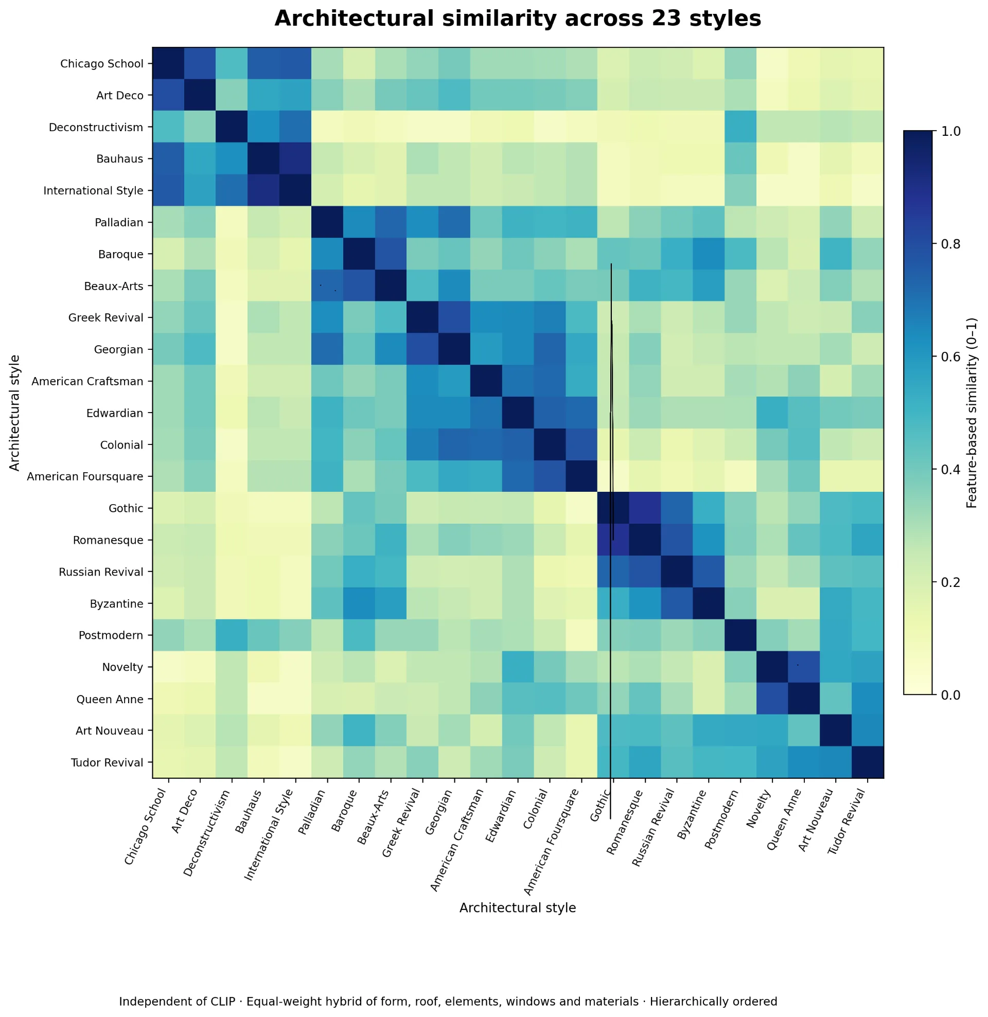
Each entry represents the architectural similarity between two styles:

Equation 14.

The matrix is symmetric: the similarity between Gothic and Romanesque is the same as the similarity between Romanesque and Gothic.

Each style also has maximum similarity with itself:

Equation 15

Excluding comparisons of a style with itself, we obtain 253 unique pairs of architectural styles:

Equation 16.

Some of the strongest relationships identified by our feature-based measure are shown below in Table 6.

Architectural Styles	Similarity
Bauhaus-International Style	0.917
Gothic-Romanesque	0.880
Greek Revival-Georgian	0.800
Novelty-Queen Anne	0.800
Chicago School-Art Deco	0.800
Colonial-American FourSquare	0.780
Baroque-Beaux Arts	0.780
Russian Revival-Byzantine	0.760

Table 6.

Several relationships are consistent with established architectural characteristics. Bauhaus and International Style share geometric simplicity and very little ornamentation. Gothic and Romanesque architecture share structural and historical features, while Greek Revival and Georgian architecture share symmetry and classical proportions.

These examples suggest that our similarity measure produces reasonable results. However, the scores depend on our choice of features and their equal weighting. Different features or weights could produce different results.

5.6 How Similar are Architectural Styles in General?

Before applying our measure to CLIP’s retrieval results, we examined the distribution of similarity scores across all 253 distinct style pairs. The mean architectural similarity was 0.345, and the median was 0.307.

The 75th percentile was 0.460, meaning that approximately three-quarters of the style pairs had similarity scores at or below that value. At the upper end of the distribution, the 90th percentile was 0.639, and the 95th percentile was 0.733. These values establish a reference distribution against which CLIP’s label mismatches can be evaluated.

A similarity score of 0.70, for example, is not merely a number between zero and one. Within our architectural similarity matrix, it represents a relatively strong relationship compared with most other architectural style pairs.

This allows us to evaluate a retrieval mismatch in context.

If CLIP retrieves a Romanesque building for a Gothic query, we can look up the architectural similarity between those styles and determine how that relationship compares with the full distribution. Instead of treating every mismatch as equally incorrect, we can begin distinguishing retrievals involving closely related styles from those involving substantially different architectural characteristics.

5.7 Two Perspectives on Architectural Similarity

CLIP measures similarity through learned image representations, while our feature-based measure compares architectural styles. Both have limitations: CLIP may be influenced by irrelevant visual details, and our measure does not compare individual buildings.

But does CLIP retrieve architecturally related styles more often than we would expect by chance?

Let’s examine the evidence.

6. When CLIP Gets It Wrong, Could It Be Right?

We now examine whether CLIP’s label mismatches reflect meaningful architectural similarities.

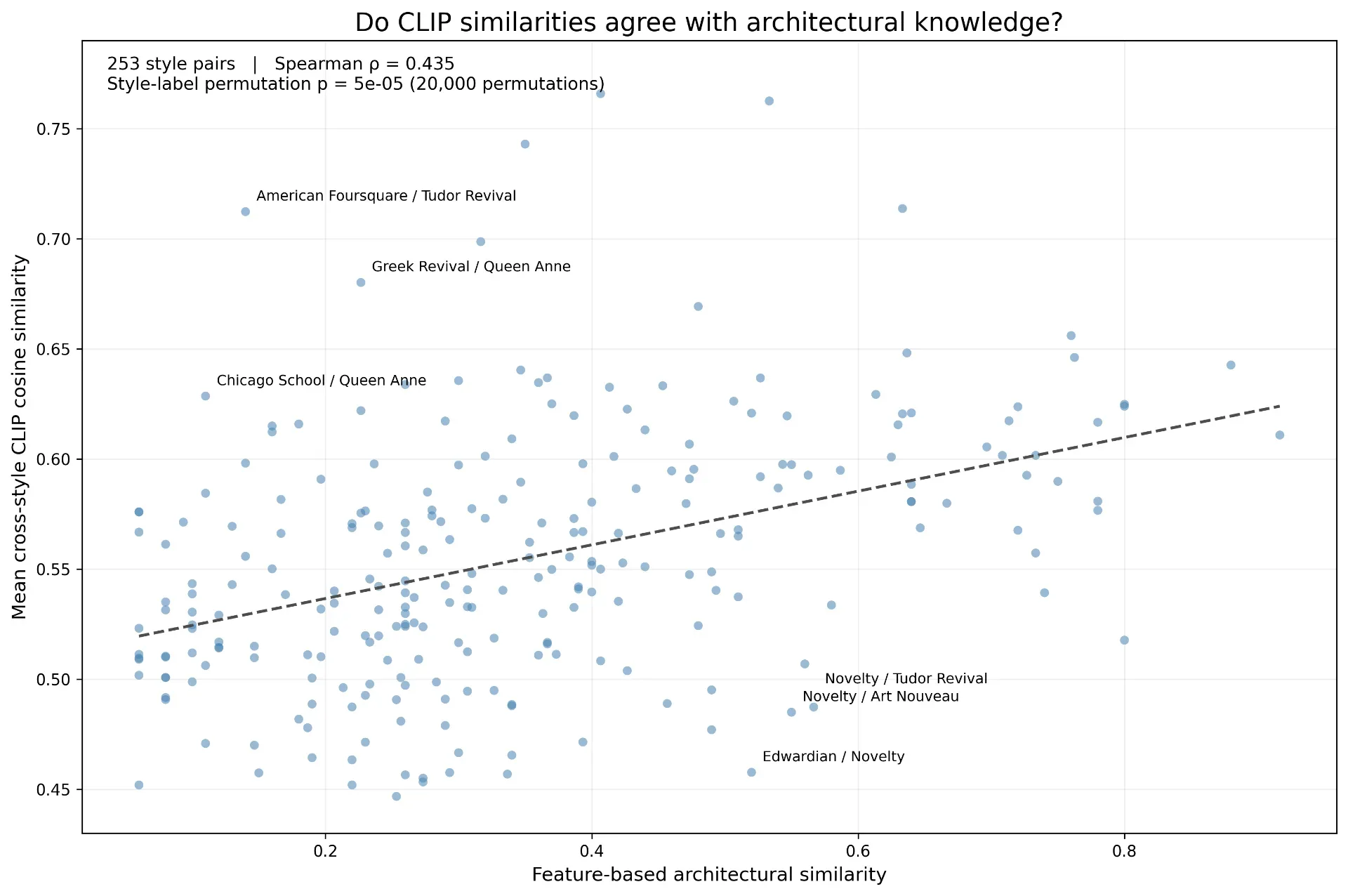
Before analyzing the retrieval results, we compared our feature-based similarity scores with the mean CLIP cosine similarity for each of the 253 unique architectural style pairs.

The results show a moderate positive correlation (Spearman ρ = 0.435). Styles with higher feature-based similarity generally receive higher CLIP similarity scores, although some pairs show substantial disagreement.

6.1 How Architecturally Similar Are CLIP’s Mismatches?

We examined CLIP’s 2,465 Precision@1 label mismatches, obtaining the similarity between each query style and its retrieved style from our architectural similarity matrix.

Let qᵢ denote the architectural style of query i, and rᵢ the style of its top-ranked retrieval.

We define the set of label mismatches as:

Equation 17.

For our dataset, $mathcal{|E|}=2,465$

For each mismatch, its architectural similarity is:

Equation 18.

where $M_{text{feature}}$

The mean architectural similarity among mismatches is:

Equation 19.

The distribution provides additional insight.

Statistic	Architectural similarity
Mean	0.500
Median	0.473
75th percentile	0.667
90th percentile	0.800
Maximum	0.917

Table 7.

These results indicate that many of CLIP’s mismatches involve styles sharing substantial architectural characteristics.

However, an absolute similarity score does not tell us how unusual that resemblance is. A score of 0.50 might be high or low depending on the similarity distribution across all architectural styles.

To put these results into perspective, we compared the architectural similarity of each mismatch with the similarity scores of all 253 distinct architectural style pairs. We then calculated the percentile rank of each mismatch and averaged these ranks. This helps us understand where CLIP’s mismatches tend to fall within the overall distribution of architectural similarities.

How did we calculate the mean percentile rank of mismatch similarity scores?

We ranked the 253 architectural style pairs according to their similarity scores. For each of CLIP’s 2,465 mismatches, we determined where its similarity score fell within this distribution.

For example, a percentile rank of 80 means that the mismatch has an architectural similarity score higher than approximately 80% of all style pairs.

We then calculated the mean percentile rank by adding the percentile ranks of all 2,465 mismatches and dividing by 2,465:

Equation 20.

where P_i is the percentile rank of mismatch i.

What did we find?

• Mean percentile rank: 71.2. On average, CLIP’s mismatches ranked around the 71st percentile in architectural similarity.

• 51.4% of mismatches fell within the top 25% of architectural similarities.

• 27.5% fell within the top 10%.

• 18.6% fell within the top 5%.

These results show that CLIP’s mismatches were concentrated among architectural styles with relatively high similarity scores, rather than being distributed uniformly across all possible style pairs.

But could this pattern arise simply because some architectural styles occur more frequently than others in our dataset?

To answer that question, we conducted a Monte Carlo experiment.

6.2 Are CLIP’s Mismatches More Meaningful Than Chance?

A convincing evaluation requires more than showing that CLIP retrieves architecturally similar styles. We must establish whether the observed similarities exceed what would be expected from random retrieval.

Importantly, our dataset does not contain equal numbers of images for every architectural style. A random retrieval is therefore more likely to return a common style than a rare one. To account for this imbalance, we constructed a frequency-aware random baseline.

For each of the 2,465 queries associated with a label mismatch, we randomly selected an alternative architectural style, excluding the query’s own style. Alternative styles were sampled proportionally to their frequencies in the dataset. We then calculated the mean architectural similarity between each query style and its randomly selected alternative.

This process was repeated 10,000 times, using a fixed random seed of 42 for reproducibility.

Let $r_i^{(b)}$

The mean similarity for that trial is:

Equation 21.

where $mathcal{|E|}=2,465$

We then compared the observed CLIP mean with the distribution of the 10,000 simulated means.

Results

Metric	Value
Observed CLIP mean similarity	0.5001
Random baseline mean	0.3500
Random baseline standard deviation	0.0037
95% simulated null interval	0.3429–0.3573
Maximum simulated mean	0.3638
Monte Carlo trials	10,000
Monte Carlo p-value	0.00009999

The observed mean architectural similarity of CLIP’s mismatches was approximately 43% higher than the random baseline. More importantly, none of the 10,000 random trials produced a mean similarity as high as CLIP’s observed value.

This result provides strong statistical evidence that CLIP’s label mismatches exhibit greater architectural similarity than would be expected from frequency-aware random selection.

We also examined whether the result was driven by a small number of frequently confused style pairs. The 2,465 mismatches involved 287 distinct directional style pairs, and the five most frequent pairs accounted for only 11.9% of the mismatches. Thus, the observed architectural resemblance was not confined to a handful of recurring style confusions.

The conclusion is significant: even when CLIP retrieves an image with the wrong architectural label, its choice is far from random in terms of architectural characteristics.

7. Discussion: Beyond Architectural Retrieval

The limitations of category-based evaluation extend beyond architectural image retrieval.

In fashion retrieval, clothes from different categories may share similar silhouettes, textures, or design elements. In product search, competing brands may offer nearly identical products. In semantic search, documents assigned to different topics may express closely related ideas.

These examples illustrate why relevance depends on the application. Visual appearance may matter most in fashion, functionality in product search, and meaning in document retrieval.

Improving retrieval systems therefore requires not only better models, but also evaluation methods that reflect what users actually consider relevant.

8. Conclusion

Using 9,315 images representing 23 architectural styles, we found that CLIP’s 2,465 label-mismatched Precision@1 retrievals showed significantly greater architectural similarity than expected under a frequency-aware random baseline, as our Monte Carlo experiment showed.

Our findings show that conventional categorical evaluation can overlook meaningful relationships captured by embedding-based retrieval systems. They support complementing Precision@K with application-specific similarity measures to provide a more complete assessment of retrieval quality.

Thank you for reading!

The dataset used in the article can be found at:

https://www.kaggle.com/datasets/dumitrux/architectural-styles-dataset

The entire code for the article can be found at:

https://github.com/theomitsa/AI-Architectural-Evaluation

Note: All figures and plots were created by the author.

Data license information: CCO: Public domain.

https://creativecommons.org/publicdomain/zero/1.0/