Jev Calibration Tested Against Scikit-Learn on BANKING77

Here is a message from the BANKING77 test set: “I lost my wallet today with all my credit cards. Will you please block the card and send a replacement?”

I gave it to a logistic regression classifier, calibrated with isotonic regression, that could choose from seven banking intents. None of the seven was “lost or stolen card”, so the right answer wasn’t on the list. The classifier picked card_payment_fee_charged with probability 0.984. A routing rule of “act above 0.90” would have treated a lost wallet as a fee question and moved on. The same logistic regression before calibration gave the same wrong label at 0.51 and would have escalated it. Calibration made the model better on average and more confident about this mistake.

On September 15, 2026, TypeSafe AI launched Jev, a model built for this kind of decision. You send it a state (a support ticket, a transaction record, a proposed tool call) plus a set of typed questions, and it returns structured answers with probabilities: a choice from a list you defined, a score on a rubric you defined, or a yes/no with a number attached. TypeSafe says the model doesn’t generate text, so there is no JSON to parse and no retry loop for malformed output [1]. (The API does report output tokens; they aren’t billed.) TypeSafe calls it a System One model, after Kahneman’s fast-versus-slow distinction [2], and says it trains with a method called RLCD, reinforcement learning for calibrated decisions. RLHF rewards answers people prefer. RLCD is supposed to reward probabilities that match reality, so that outcomes assigned 0.2 happen about 20% of the time [1].

When I ran these tests, TypeSafe had published no paper and no weights, and Jev was available only through its API, with input billed at $0.042 per million tokens and output free [1]. So I asked two questions. Can open tooling reproduce Jev’s contract (typed questions, probabilities you can check, and abstention as a branch your code can take)? And what does the real API add? I rebuilt the contract on scikit-learn, measured how calibrated small open models are, whether calibration makes a confidence-gated cascade cheaper, and where the typed interface breaks, then ran the same harness against Jev.

All numbers here are from my own runs unless they’re cited. Details about Jev itself come from TypeSafe’s documentation [1], and the cascade costs in Experiment 2 are my assumptions.

In short: on the 7-intent slice, a temperature-scaled logistic regression and Jev’s Choice answers are calibrated about equally well (ECE 0.022 vs. 0.014; a paired bootstrap can’t tell them apart). On the full 77-intent task, the open model is better calibrated (0.031 vs. 0.065). Jev gets there without training, using at most three labeled examples per intent in the prompt; my models trained on 10,003 labeled queries. Jev’s yes/no answers are underconfident on true cases. The none-of-the-above trap reproduces on open models and on Jev. So does the framing inconsistency, and on both, most of its raw size comes from comparing two differently calibrated numbers at one threshold.

How Jev works, and how I rebuilt it

Jev’s API has three question types [1]. A Choice picks from up to 255 options you define and returns the full distribution. A Score takes an ordered set of levels and returns the expectation, which can land between two levels. A Noul (TypeSafe’s word for a yes/no truth question) returns P(true). Every answer also carries a confidence value. That number describes how concentrated the distribution is, and it is separate from the top probability.

I reimplemented the contract over plain scikit-learn classifiers. The question and answer types are dataclasses:

from dataclasses import dataclass@dataclassclass ChoiceQuestion:    name: str    instructions: str    criteria: dict  # option -> description string@dataclassclass ChoiceAnswer:    choice: str    probabilities: dict    confidence: float  # concentration of the distribution, 0..1

A backend is anything that maps (state, questions) to answers. The open backend wraps any fitted classifier that has predict_proba (simplified here; the full version is in the repo):

class SklearnBackend(Backend):    def __init__(self, clf, vectorizer=None):        self.clf = clf        self.vectorizer = vectorizer    def answer(self, state, questions):        X = self.vectorizer.transform([state])        proba = self.clf.predict_proba(X)[0]        classes = list(self.clf.classes_)        out = {}        for q in questions:            options = list(q.criteria.keys())            probs = {opt: float(proba[classes.index(opt)])                     for opt in options if opt in classes}            total = sum(probs.values()) or 1.0            probs = {k: v / total for k, v in probs.items()}            top = max(probs, key=probs.get)            out[q.name] = ChoiceAnswer(                choice=top, probabilities=probs,                confidence=_concentration_confidence(list(probs.values())))        return out

For confidence I used one minus normalized entropy: 1.0 when all the mass sits on one option, 0.0 when the distribution is uniform. Because the real Jev slots in as a second backend behind the same signature, the application code (thresholds, escalation, logging) never touches model internals and only branches on the numbers that come back.

Experiment 1: how well calibrated are small open models?

I measured Expected Calibration Error (ECE) and Brier score on BANKING77 [3], a 77-intent dataset of banking queries (10,003 train, 3,080 test), and on a 7-intent slice made of the seven most frequent intents in the training set (280 test queries). All four classifiers share the same features, TF-IDF over unigrams and bigrams with up to 20,000 terms:

• multinomial Naive Bayes

• logistic regression (C = 4)

• the same logistic regression with per-class isotonic calibration (scikit-learn’s CalibratedClassifierCV, 3 folds)

• the same logistic regression with a single temperature fit on out-of-fold logits

ECE [4] groups predictions into bins by their top probability and averages the gap between confidence and accuracy in each bin, weighted by bin size:

ECE = Σ_b (|B_b| / n) · |acc(B_b) − conf(B_b)|

Here B_b is the set of predictions whose top probability falls in bin b, acc(B_b) is the share of them that are correct, and conf(B_b) is their mean top probability. A perfectly calibrated model scores 0. I use 15 equal-width bins everywhere in this article, for the open models and for Jev. In code:

def expected_calibration_error(y_true, y_prob, n_bins=15):    """ECE with equal-width bins: sum_b |acc(b) - conf(b)| * |b| / n."""    bins = np.linspace(0.0, 1.0, n_bins + 1)    ece = 0.0    for lo, hi in zip(bins[:-1], bins[1:]):        mask = (y_prob > lo) & (y_prob <= hi) if lo > 0 else (y_prob >= lo) & (y_prob <= hi)        if mask.sum() == 0:            continue        ece += (mask.sum() / len(y_true)) * abs(y_true[mask].mean() - y_prob[mask].mean())    return float(ece)

The Brier score here is the squared error between the top probability and whether the top label was right, averaged over queries.

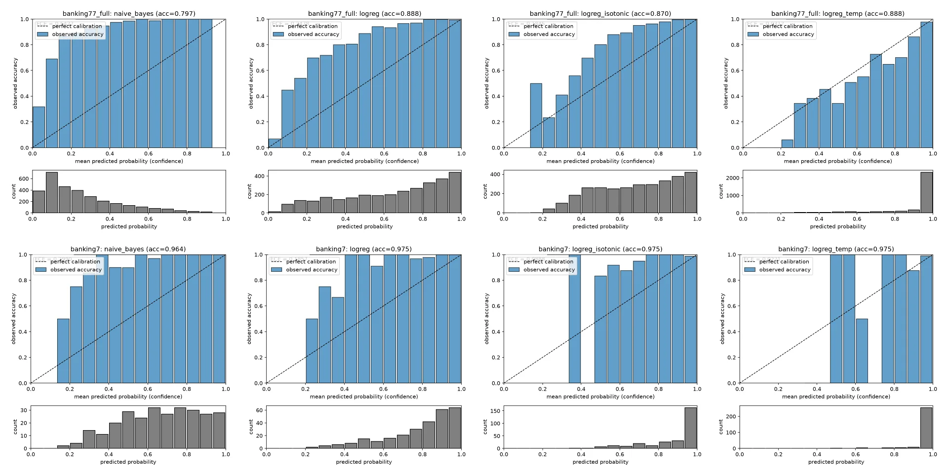
Naive Bayes reaches 80% accuracy on 77 intents while its probabilities are close to meaningless (ECE 0.54). The direction surprised me. I expected overconfidence, which is what the textbooks say about Naive Bayes [5], and got the opposite: its mean top probability is 0.25 against 0.80 accuracy. My guess is that with 77 classes of short text, TF-IDF Naive Bayes spreads its probability mass thin. Plain logistic regression is underconfident too, with a mean top probability of 0.64 against 0.89 accuracy. Underconfidence costs you in wasted escalation rather than wrong actions, as Experiment 2 shows.

Isotonic and temperature scaling gave very different results on the same task. Per-class isotonic calibration [6] cost 1.7 points of accuracy on 77 intents and still left ECE at 0.185. Fitting 77 separate calibration maps and renormalizing can re-rank classes and change predictions, which made it the wrong tool here. A single temperature [7] took ECE to 0.031 with no accuracy cost. Temperature scaling divides the model’s logits z by one learned number T before the softmax:

p_k = exp(z_k / T) / Σ_j exp(z_j / T)

T > 1 flattens the distribution and T < 1 sharpens it. Dividing every logit by the same positive number can’t change which one is largest, so accuracy stays at 0.888 by construction. On the 7-intent slice, isotonic cost nothing and halved ECE, and temperature took it to 0.022.

The temperature is fit by minimizing negative log-likelihood on out-of-fold logits: each training query’s logits come from a model that didn’t see it, so the base model can still train on all the data.

class TemperatureScaledLR:    def fit(self, X, y):        self._lr = LogisticRegression(max_iter=1000, C=4.0).fit(X, y)        self.classes_ = self._lr.classes_        # Out-of-fold logits: T is fit on data the model didn't see.        oof = np.zeros((len(y), len(self.classes_)))        for tri, cai in StratifiedKFold(n_splits=3, shuffle=True,                                        random_state=7).split(X, y):            m = LogisticRegression(max_iter=1000, C=4.0).fit(X[tri], y[tri])            oof[cai] = m.decision_function(X[cai])        cidx = np.where(self.classes_[None, :] == y[:, None])[1]        def nll(T):            z = oof / T            z = z - z.max(axis=1, keepdims=True)            p = np.exp(z) / np.exp(z).sum(axis=1, keepdims=True)            return -np.log(p[np.arange(len(y)), cidx] + 1e-12).mean()        self.temperature_ = minimize_scalar(nll, bounds=(0.05, 20.0),                                            method="bounded").x        return self    def predict_proba(self, X):        z = self._lr.decision_function(X) / self.temperature_        z = z - z.max(axis=1, keepdims=True)        return np.exp(z) / np.exp(z).sum(axis=1, keepdims=True)

In Figure 1, before calibration, mean confidence sits below accuracy in most bins. If your policy is “act above 0.9”, only the predictions above 0.9 matter, so look at those bins directly instead of trusting the average.

Experiment 2: does calibration make a cascade cheaper?

The economic pitch for decision models is a cascade. The cheap model acts when it’s confident and escalates the rest to a frontier model or a person. The escalation decision runs on the confidence score, so I tested the policy on the full 77-intent task with three backends: Naive Bayes (ECE 0.54), plain logistic regression (ECE 0.25), and the same logistic regression with temperature scaling (ECE 0.03). The last two make identical predictions, so comparing them nearly isolates calibration from ranking. Temperature scaling can still slightly reorder top probabilities across queries, which accounts for the small gap between them below.

The policy is one comparison. If the top probability clears a threshold t, auto-decide. Otherwise, escalate. Coverage is the share of traffic the cheap model decides on its own. I assumed the escalation tier is 97% accurate and costs 100 times the cheap tier. Both numbers are assumptions I chose. What I measured is how precision, coverage and cost trade off under each model’s own scores:

FRONTIER_ACC = 0.97   # assumed accuracy of the escalation tierCOST_RATIO = 100.0    # assumed cost of escalation vs. the cheap tierdef cascade_point(top_p, correct, t):    auto = top_p >= t    cov = auto.mean()    prec = correct[auto].mean()    esc = 1.0 - cov    return {"coverage": cov,            "precision_auto": prec,            "overall_acc": cov * prec + esc * FRONTIER_ACC,            "rel_cost": cov * 1.0 + esc * COST_RATIO}

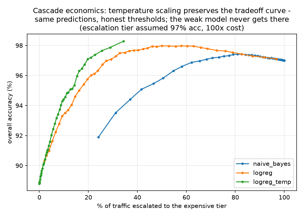
The table reads differently depending on whether you fix a precision target or a threshold.

The first column fixes a precision target of 95% on auto-decided queries and asks how much each model must escalate to hit it. That is mostly a test of ranking, because each model gets its own threshold and underconfidence washes out. Plain and temperature-scaled logistic regression escalate 18.1% and 14.1%, close as you’d expect from near-identical orderings. Naive Bayes needs 51.7% because it ranks worse. I computed these operating points exactly, trying every distinct score as a cutoff, but the thresholds come from the test set. They are oracle numbers. In production you’d pick them on a validation split.

The second column fixes the threshold at 0.90, the number you’d write in a config file. Naive Bayes auto-decides 0.2% of traffic at 100% precision. It is never wrong and almost never acts, at 99.8 times the base cost. Plain logistic regression auto-decides 21.1% at 99.5% precision. The temperature-scaled model auto-decides 78.9% at 97.2%.

For the calibrated model, the mean confidence of the queries it acts on is 0.989, which predicts 98.9% precision. Measured precision is 97.2%, so above 0.90 the model is 1.7 points overconfident. Temperature scaling fixed the average and flipped the error at the top from timid to slightly optimistic, because one global temperature can’t fit every bin at once. For plain logistic regression, the same calculation predicts 94.9% against 99.5% measured. That error is in the safe direction, and it’s why the uncalibrated policy is safe and timid, acting on about a fifth of the traffic.

Calibration is supposed to let you pick a threshold without labels. If the scores are honest, the threshold where the mean confidence of acted-on queries reaches 0.95 should give you about 95% precision:

def unlabeled_threshold_for_target(top_p, target):    """Smallest t whose acted-on items have mean confidence >= target."""    s = np.sort(top_p)[::-1]    cummean = np.cumsum(s) / np.arange(1, len(s) + 1)    ok = np.where(cummean >= target)[0]    return float(s[ok[-1]]) if len(ok) else None

On the calibrated model this gives t ≈ 0.54, and measured precision there is 92.4%. The labeled answer was 0.78. I expected the shortcut to land near 0.78, since the model had looked only 1.7 points optimistic above 0.90. Over the whole range the shortcut acts on (0.54 to 1.0), its confidence averages 2.6 points above its accuracy. For plain logistic regression the shortcut gives t ≈ 0.90 with measured precision 99.5%, 4.5 points over the target in the safe direction. The threshold that buys exactly 95% precision there is 0.34, and you can only find that with labels.

I left isotonic out of this experiment. On the 77-intent task it escalated 23.5% at the 95%-precision point, against 18.1% for the uncalibrated model, so it made ranking worse as well as costing accuracy.

With calibrated scores, a fixed threshold gets you close to a target precision without labels: 2.6 points short here. A hard precision SLA still needs a labeled check. If you buy a model for a cascade, its calibration is what decides how much traffic it can handle alone, which is the case TypeSafe makes for training on calibration with RLCD.

Experiment 3: where the typed interface breaks

A typed interface has two obvious ways to fail. One is the none-of-the-above trap: a Choice question has to pick an option even when none fits. The other is the framing inconsistency: the same question asked two ways, as a Choice and as a Noul, can come back with probabilities that don’t agree. I tested both on open models first, to see whether they belong to one vendor or to the paradigm.

The none-of-the-above trap

I asked the 7-intent classifier about 600 queries drawn from the other 70 intents, so the true answer was never among the options. My isotonic-calibrated 7-intent model did lower its confidence on these inputs (mean top probability 0.70 out of schema vs. 0.89 in schema), but not enough. At a threshold of 0.90 it auto-acted on 21.2% of them. Every one of those actions was wrong by construction.

Then I reran the trap with the temperature-scaled backend, which is better calibrated in distribution (ECE 0.022 on this slice). At the same 0.90 threshold, false auto-acts rose from 21.2% to 29.2%. I wrote “the trap got worse” in my notes. The operating point had moved, though. In-schema auto-acts rose from 65.7% to 92.1% in the same step, and the ratio of false acts to in-schema acts was about 0.32 for both models.

The fair comparison is at matched in-schema coverage: pick each model’s threshold so it acts on the same share of in-schema traffic, then count out-of-schema actions.

def out_act_at_coverage(p_in, p_out, coverage):    t = float(np.quantile(p_in, 1 - coverage))   # threshold giving this coverage    return t, float((p_out >= t).mean())          # false auto-act rate at that tfor cov in (0.50, 0.657, 0.80, 0.90, 0.921):    t_iso, out_iso = out_act_at_coverage(pin_iso, pout_iso, cov)    t_tmp, out_tmp = out_act_at_coverage(pin_tmp, pout_tmp, cov)

At 65.7% in-schema coverage, the temperature-scaled model wrongly acts on 3.5% of out-of-schema inputs, against 21.2% for the isotonic model. Its threshold there is 0.9989, against 0.9004 for isotonic. The pattern held at every coverage level I checked, and the gap between in-schema and out-of-schema mean confidence widened from 0.19 to 0.26. So the sharper model separates the two groups better, but only at a threshold you would not pick without labeled data.

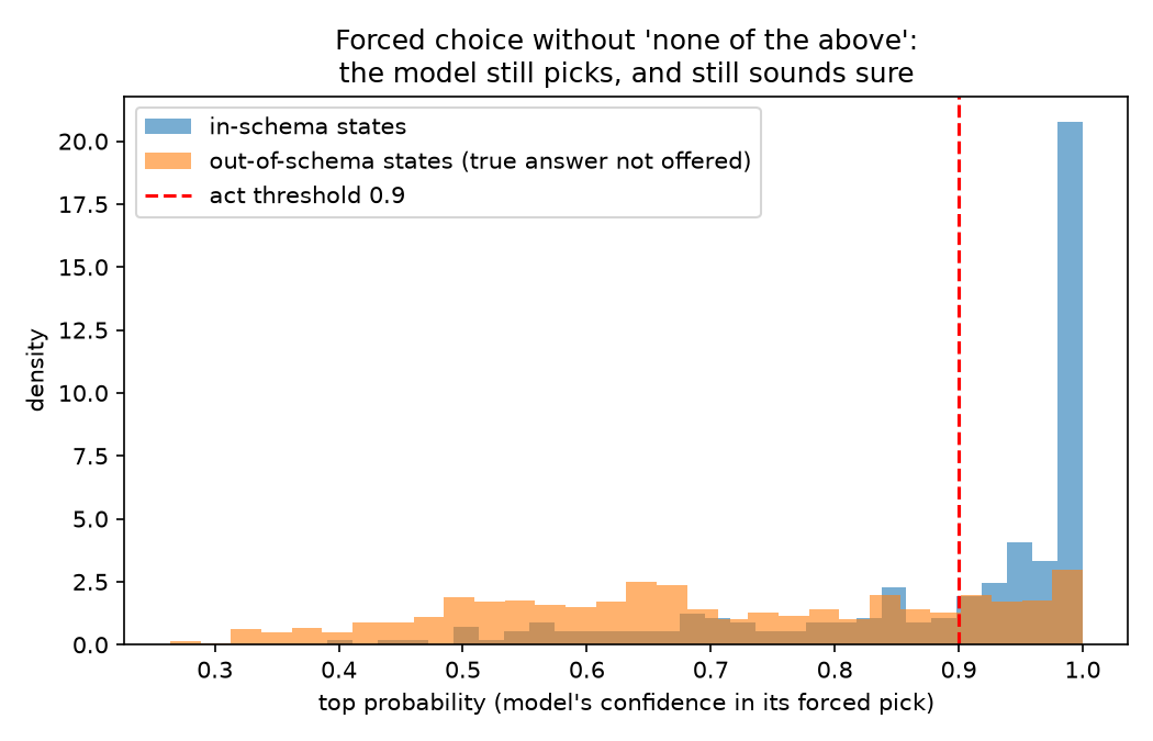
At the deployed 0.90 threshold, the temperature-scaled model still acts on 29% of out-of-schema inputs.

The schema needs a way out. One way is a threshold below which the system abstains or routes the query to “none of these”:

act = top_p >= thresholdif act:    branch = "ACT"elif none_branch:    branch = "NONE_OF_THESE"else:    branch = "ABSTAIN"

With the threshold at 0.9989, the lost-wallet message from the top of this article (top probability 0.981 on the temperature-scaled model) routes to NONE_OF_THESE instead of being filed as a fee question. That threshold came from labeled data, though. The other way out is an explicit “none of these” option in the Choice question itself. I didn’t test that, on open models or on Jev.

The framing inconsistency

Jev answers each question in isolation [1], so nothing makes two framings of the same question agree. A Choice and a Noul about the same intent can each be well calibrated and still land on opposite sides of an action threshold.

To reproduce it on open models, I used the same protocol I later ran on Jev. For each of the 280 queries in the 7-intent slice, the Choice framing is the multiclass model’s top probability. The Noul framing is a separate one-vs-rest logistic regression’s P(true) for the intent the Choice picked. The two contradict when one clears 0.90 and the other doesn’t.

The one-vs-rest classifiers are more cautious than the multiclass model: at 0.90 they act on 27.5% of queries, against 35% for plain and 92% for temperature-scaled logistic regression. Temperature scaling sharpens the Choice framing, so the two framings drift apart at a fixed threshold even though they mostly agree on the answer. Matching the action rates (picking the Noul threshold that acts on as many queries as the Choice framing does) removes most of the gap. Two answers to the same question, calibrated separately, are two different numbers. That holds for open models too, so the inconsistency belongs to the paradigm and not only to Jev.

My first version of this test was looser: one target intent over all 77 classes. There, both framings almost never cleared 0.90, so they almost never disagreed (0.03%). I’m mentioning it because a test where nothing acts can’t show a contradiction.

Experiment 4: the same tests on the real Jev API

Everything above runs on open models. TypeSafe’s central claim, calibrated probabilities with no training, belongs to Jev, so I ran the same harness against the live API. On the 280-query banking slice, each call carried one Choice question plus seven Noul questions, one per intent:

INTENTS = {    "card_payment_fee_charged":        "The customer was charged a fee for paying with their card and is asking about or disputing it.",    "transaction_charged_twice":        "The same transaction appears twice on the statement; the customer was charged a duplicate amount.",    # ... five more intents}questions = {"intent": {    "type": "choice",    "instructions": "Classify this customer support message into exactly one of the listed intents.",    "criteria": INTENTS,}}for intent, desc in INTENTS.items():    questions[f"noul_{intent}"] = {        "type": "noul",        "instructions": "This customer message matches the following situation: " + desc,    }body = {"model": "jev-latest", "state": text, "questions": questions}# POST https://api.typesafe.ai/v1/systemone

The API served jev-1.13.0 for every call. Besides the 280 banking calls, 100 calls ran the out-of-schema trap and 6,160 ran the full 77-intent task twice, once with terse criteria and once with few-shot criteria. That is 6,540 calls in total, for $0.80.

Calibration by question type

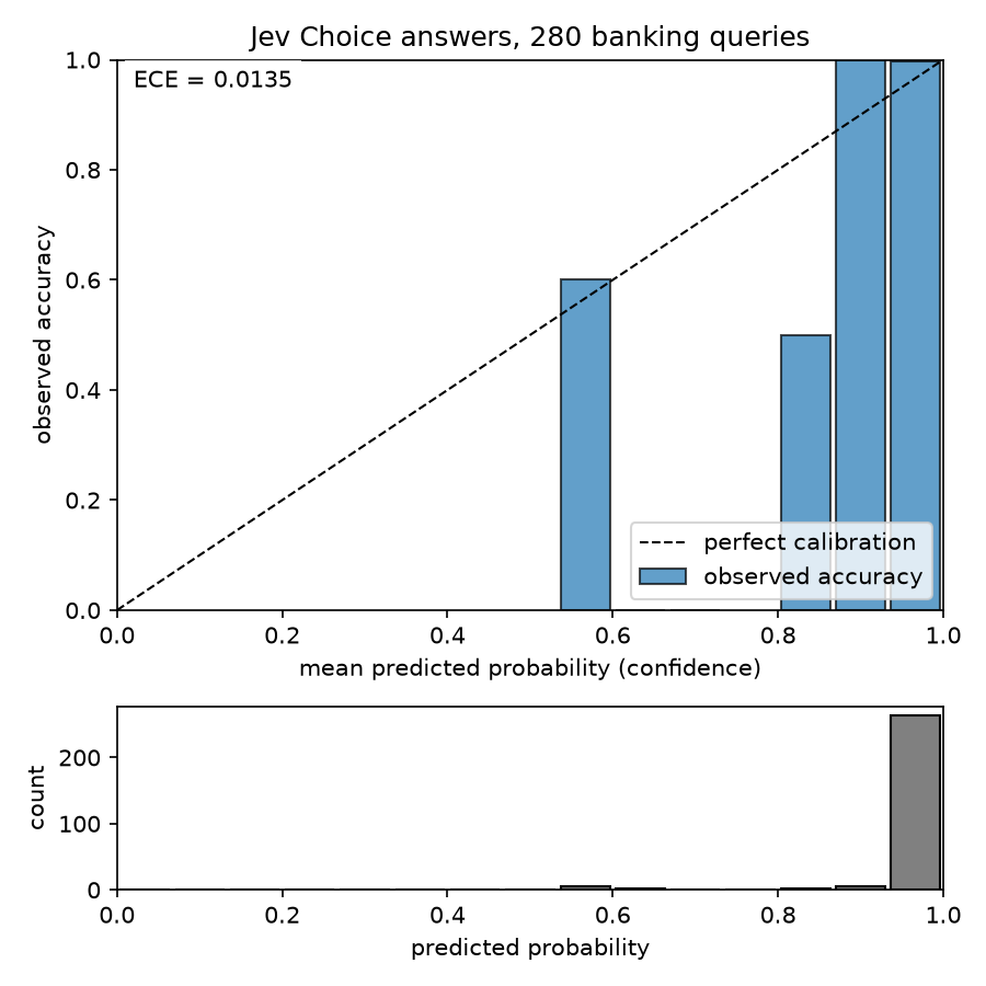
Jev’s Choice answers are very well calibrated: accuracy 0.975, ECE 0.014 (95% bootstrap interval 0.008 to 0.031), Brier 0.015 on 280 queries. My temperature-scaled model scored 0.022 on the same queries. A paired bootstrap of the difference, resampling the same queries for both models, gives 0.008 with an interval of −0.004 to 0.020, so I can’t call the two different. Jev is also decisive: 85% of its Choice answers put more than 0.99 on one option.

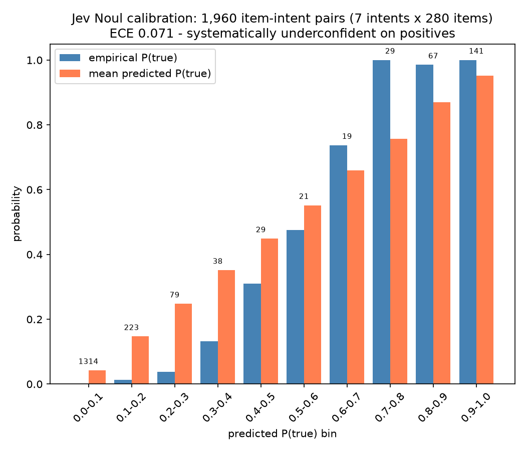
Jev’s Noul answers are underconfident on true cases. Across the 280 query-intent pairs where the answer is yes, mean P(true) is 0.84, and only 56% of those pairs clear 0.9. On the 1,680 pairs where the answer is no, Noul is close to perfect. The pooled ECE over all 1,960 pairs is 0.071 (interval 0.067 to 0.078, resampling by query), but that number mostly reflects the easy negatives. I didn’t compute the same yes/no calibration for my open models, so I make no open-vs-Jev claim for Noul.

Accuracy on all 77 intents

I also ran Jev on all 3,080 test queries with 77 options, once with terse criteria derived from the intent names (“card payment fee charged”) and once with three example queries per intent written into the criteria text. The examples were the three training queries closest to each intent’s TF-IDF centroid, so none came from the test set. Terse criteria gave accuracy 0.801 and ECE 0.083. Three-shot criteria gave 0.859 and 0.065.

The temperature-scaled open model scores 0.888 and 0.031 on the same task, so Jev holds no calibration lead here. Three-shot Jev trails supervised logistic regression by about 3 points of accuracy, and terse Jev trails by about 9 (it does edge out Naive Bayes at 0.797). The supervised models fit weights on 10,003 labeled queries. Jev saw 77 short phrases, then 231 example queries as description text, with no training step. Better descriptions closed 6 of the 9 points and cut ECE from 0.083 to 0.065. I didn’t test whether richer descriptions would close the rest. If Jev saw BANKING77 during training, these accuracies are ceilings.

Latency and cost

I measured latency on my side, as wall-clock time per request, with eight requests in flight for the 7-intent run. Median latency was 0.37 seconds per call with eight questions in it, and p95 was 0.61 seconds. The first eight calls each took about 16 seconds, which looks like warm-up; after them, no call in that run took longer than 0.7 seconds. Single-question calls with 77 options had about the same median (0.36 seconds), which is consistent with TypeSafe’s claim that questions in one request are evaluated in parallel [1]. I didn’t test that claim directly.

Computed from the reported input tokens at list price, the 7-intent calls (eight questions each) cost about 3.4 cents per thousand. The 77-option calls cost 7.1 cents per thousand with terse criteria and 18.3 cents with three-shot criteria, because each call carries far more input tokens. Across all 6,540 calls it came to about 12 cents per thousand. I didn’t run Jev through the Experiment 2 cascade, so its latency and price look compatible with a cascade, but I can’t say what its cascade curve looks like.

The two failure modes on Jev

The framing inconsistency reproduces. I asked “which intent is this?” as a Choice and “is this intent X?” as a Noul for each of the seven intents. At t = 0.90 the two framings disagreed on act versus abstain for 111 of 280 queries (39.6%). Every contradiction ran the same way: Choice said act and Noul said abstain. Because Noul is underconfident on true cases, it acts on only 56% of queries at 0.90, while Choice acts on 96%. Matching the action rates (a Noul threshold of 0.44) drops the disagreement to 6.4%, 18 of 280 queries, nine in each direction. That is in the same range as my open models under the same protocol (2.9% and 5.0%). If you threshold one framing’s numbers, don’t mix in the other’s.

The none-of-the-above trap reproduces too. On 100 out-of-schema queries, Jev’s mean top probability was 0.71, close to my open models’ 0.70 and 0.72. It auto-acted on 26% of them at t = 0.90 (95% interval 17% to 35%), all wrong by construction. Jev acts on about 96% of in-schema queries at that threshold, which is closest to the temperature-scaled backend’s 92.1%, so the like-for-like comparison is Jev’s 26% against 29.2%. The samples differ (Jev’s 100 queries came from the test split, the open models’ 600 from the training split of the other intents), and given the interval, the two are about the same.

Limitations

• Everything runs on one dataset of short English banking queries, with TF-IDF features. Other domains, longer inputs and stronger open models could change every number.

• The open models are from one run with fixed seeds. I didn’t measure variance across seeds or splits. Rerunning Experiment 1 with a newer scikit-learn version moved the 77-intent numbers by up to 0.005; the 7-intent numbers reproduce exactly.

• The Jev samples are small: 280 in-schema queries and 100 out-of-schema queries.

• The Experiment 2 operating points are picked on the test set.

• I never tested Score questions, an explicit “none of these” option, or Jev inside a cascade.

• If Jev saw BANKING77 in training, its accuracy numbers are optimistic.

• Every open model here was trained on 10,003 labeled queries. Jev’s advantage is needing none. The comparison I didn’t run, and the most useful next one, is an open zero-shot or few-shot model (a natural-language-inference classifier, or a small open LLM’s label probabilities) against Jev.

Conclusion: lessons for production systems

1. Measure calibration on your own workload, per question type, over the bins your thresholds use. Calibrate with a method that can’t move your predictions. A single temperature fit on out-of-fold logits costs no accuracy by construction, while per-class isotonic calibration cost 1.7 points on the 77-intent task and still left the model underconfident. On Jev, Choice answers were far better calibrated than Noul answers on true cases, so where a dimension can be a Choice question, I’d make it one and check any Noul against my own labels.

2. Don’t treat a threshold as a policy until you know what the scores behind it are worth. The same 0.90 auto-decided 0.2%, 21.1% or 78.9% of traffic depending on the backend, and even on the calibrated model the threshold picked without labels landed 2.6 points short of its precision target. Pick thresholds on labeled data, and set them per decision against the cost of being wrong.

3. Give the schema a way out. Without one, 29% of out-of-schema queries got auto-acted on by my temperature-scaled model and 26% by Jev. Better calibration changed the operating point but didn’t close the trap, because tuning a threshold can’t add a branch that isn’t there.

4. Ask each question once, in one framing. Two framings of the same question are calibrated separately, on open models and on Jev, and at a shared threshold they disagree on up to two thirds of queries.

Jev’s contribution is the contract: typed questions in, checkable probabilities out, and abstention as a branch your code can take. On this benchmark, a temperature-scaled logistic regression matched Jev’s Choice calibration on the 7-intent slice (ECE 0.022 vs. 0.014, not distinguishable) and beat it on the 77-intent task (0.031 vs. 0.065). What the API adds is getting there without training, with at most three labeled examples per intent in the prompt, at about a third of a second per call.

All open-model experiments ran on a 2-CPU VM with scikit-learn, and total compute was minutes. Seeds: 7 for cross-validation, the bootstrap and the Jev trap sample; 0 for the open trap sample. Code, figures and raw result JSONs are at https://github.com/ankur287/jev-open-calibration. BANKING77 is the PolyAI intent dataset (CC-BY 4.0).

References

[1] TypeSafe AI, Jev documentation (2026), https://docs.typesafe.ai

[2] D. Kahneman, Thinking, Fast and Slow (2011), Farrar, Straus and Giroux

[3] I. Casanueva, T. Temčinas, D. Gerz, M. Henderson and I. Vulić, Efficient Intent Detection with Dual Sentence Encoders (2020), 2nd Workshop on NLP for Conversational AI, ACL 2020

[4] M. P. Naeini, G. F. Cooper and M. Hauskrecht, Obtaining Well Calibrated Probabilities Using Bayesian Binning (2015), AAAI 2015

[5] A. Niculescu-Mizil and R. Caruana, Predicting Good Probabilities with Supervised Learning (2005), ICML 2005

[6] B. Zadrozny and C. Elkan, Transforming Classifier Scores into Accurate Multiclass Probability Estimates (2002), KDD 2002

[7] C. Guo, G. Pleiss, Y. Sun and K. Q. Weinberger, On Calibration of Modern Neural Networks (2017), ICML 2017