Don’t Let Messy Data Bend Your Curves

When a Straight Line Stops Being Enough

Linear regression earns its popularity for good reasons: it is simple, fast, interpretable, and often surprisingly effective. But real relationships do not always cooperate with straight lines.

Some bend gradually. Some flatten. Some change behavior across different regions. Braking distance, crop response, wind-turbine power, and satellite Doppler all provide familiar examples where curvature is part of the underlying relationship rather than a nuisance to be ignored.

The previous article in this series kept the model deliberately simple and focused on robustness. I compared OLS with Huber regression [1], RANSAC [2], GNC-GM, GNC-TLS [3], and ASOR [4] to see what happens when contaminated observations try to pull a straight-line fit away from the nominal relationship.

Now we keep that same robustness problem—but give the model more room to move.

From Straight Lines to Flexible Curves

The natural first step beyond a line is to introduce polynomial features. Then we encounter a new limitation: polynomial flexibility is global, so changing one coefficient can reshape the curve everywhere. Splines offer another route by introducing flexibility locally.

That gives us two very different questions to address: which observations should the estimator trust, and what shapes should the model be capable of representing?

The estimator controls trust. The basis controls shape.

The first question is easiest to see visually. Figures 1 and 2 show a simple nonlinear example in which OLS closely follows the underlying relationship when the observations are clean, while a robust estimator remains much closer to the nominal curve when the data are contaminated.

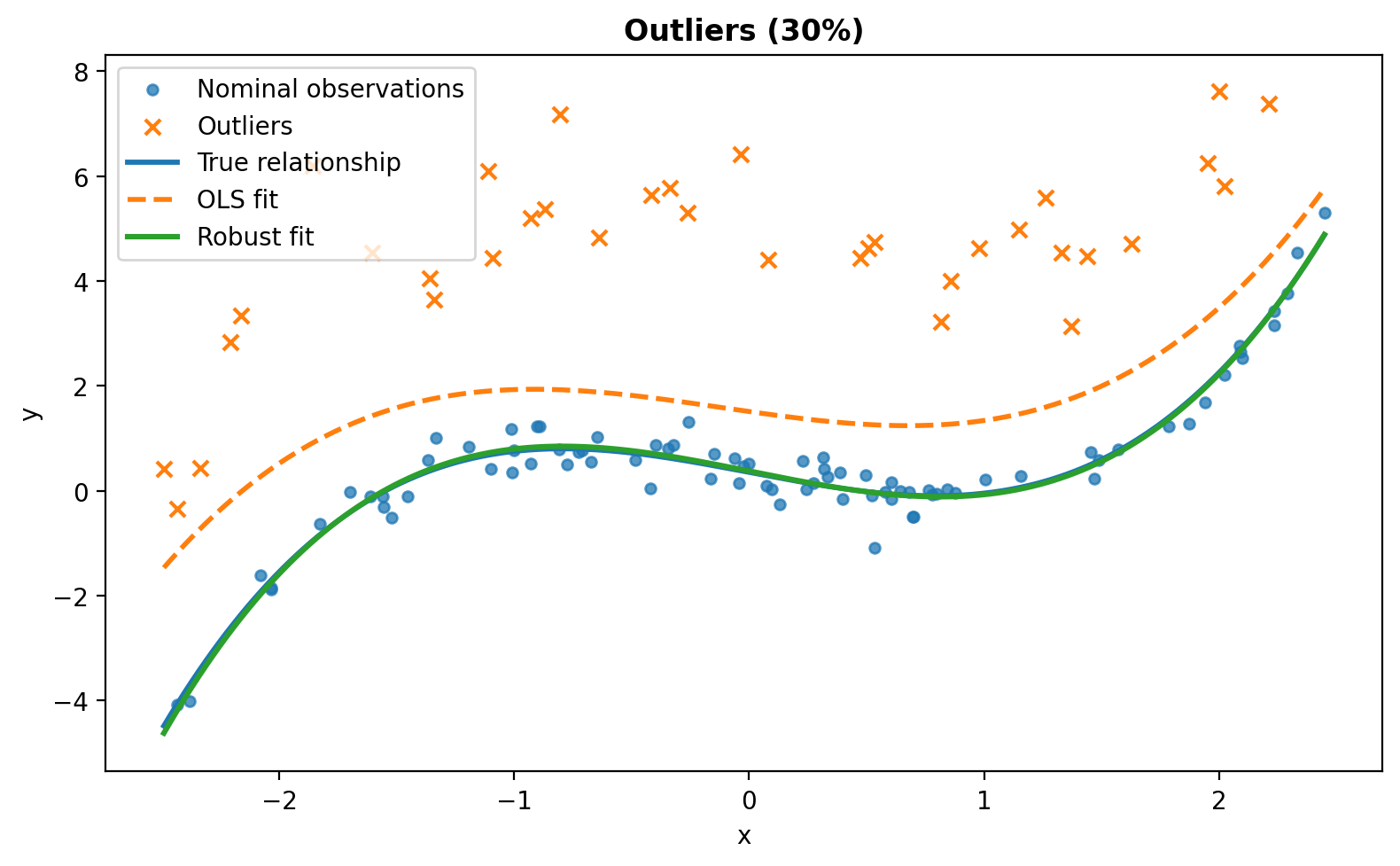
After 30% of the responses are contaminated, the OLS fit is pulled away from the underlying nonlinear relationship, while the robust fit remains much closer to it.

The second question is about representation: how do we give the model enough flexibility to describe a curved relationship? We begin with polynomial regression.

Polynomial Regression Through a Linear-Model Lens

Consider $N$ measurements, where the $i$-th measurement is modeled as

Here, the coefficients $β_k$

The measured response $y_i$

More generally,

Polynomial regression is therefore a linear model in a transformed feature space [5].

By stacking the individual measurements, the model can be written in matrix form as,

where, for a quadratic model,

OLS solves

In code, moving from a line to a polynomial is only a change in the design matrix:

def polynomial_design(x, degree):    x = np.asarray(x, dtype=float)    return np.vander(x, N=degree + 1, increasing=True)Phi = polynomial_design(x, degree=3)beta = np.linalg.lstsq(Phi, y, rcond=None)[0]

For numerical stability, especially as the polynomial degree increases or the $x_i$

Centering shifts the predictor so that its average is near zero, while scaling divides by a measure of its spread so that its values are typically of order one. The polynomial terms are then constructed from this transformed predictor, which keeps higher-order powers from becoming excessively large and improves numerical stability.

The important point is that nothing fundamental has changed. For a line, the $i$-th row of the design matrix is

while for a quadratic it becomes

The same idea extends to higher-order polynomials by adding higher powers of $x_i$

Figure 3 makes this basis expansion visible. Starting from the constant and linear terms, higher powers of the predictor are added to give the model progressively more flexibility.

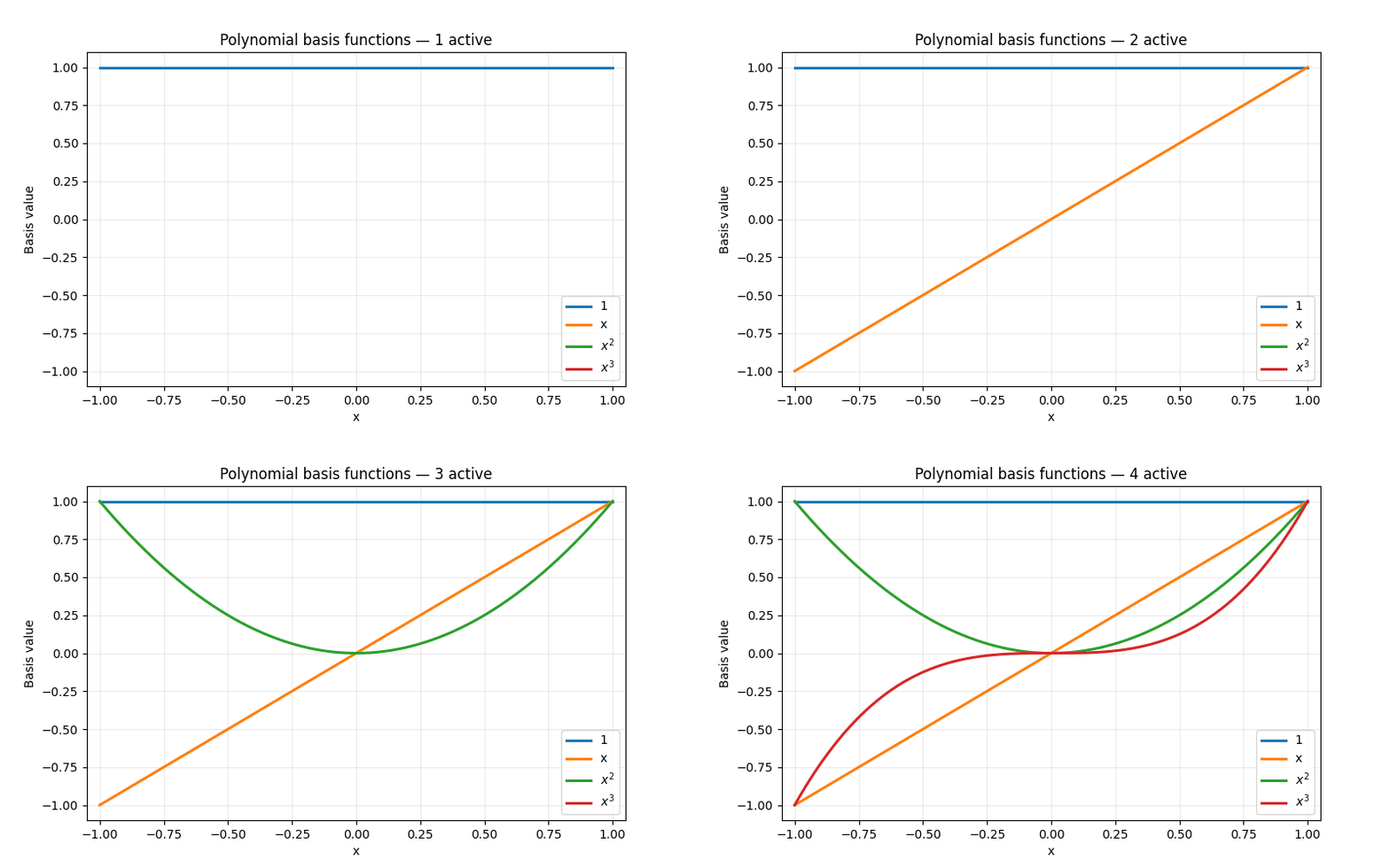
But greater flexibility comes with trade-offs. A degree-$p$ polynomial has $p+1$

That global nature is precisely where splines become useful: they provide flexibility locally rather than forcing one polynomial to explain everything at once.

When One Global Polynomial Is Not Enough

Splines introduce flexibility differently. Instead of representing the entire relationship with one global polynomial, they join polynomial pieces at selected locations called knots.

B-splines provide a convenient basis for constructing these piecewise-polynomial curves while maintaining smooth connections between neighboring pieces [7].

The spline model can be written as

where $B_{j,p}(x)$

How the B-Spline Basis Is Formed

A B-spline basis is determined by the spline degree and the knot locations.

Suppose the observed range is $[a,b]$ the spline degree is $p$ and we choose $K$ interior knots $kappa_1,kappa_2,ldots,kappa_K$

The number of resulting basis functions is $M=K+p+1$

These basis functions are constructed from the knot vector using the Cox–de Boor recursion [7]. The recursion begins with the degree-zero basis functions,

Here, $t_j$

For the quadratic spline used here,

where a term is taken as zero whenever its denominator is zero.

The basis is therefore built progressively as

The degree-zero functions are piecewise constant, the degree-one functions are piecewise linear, and the final $B_{j,2}(x)$

Figure 4 visualizes this recursive construction. The lower-degree functions are intermediate steps used to generate the final quadratic B-spline basis functions.

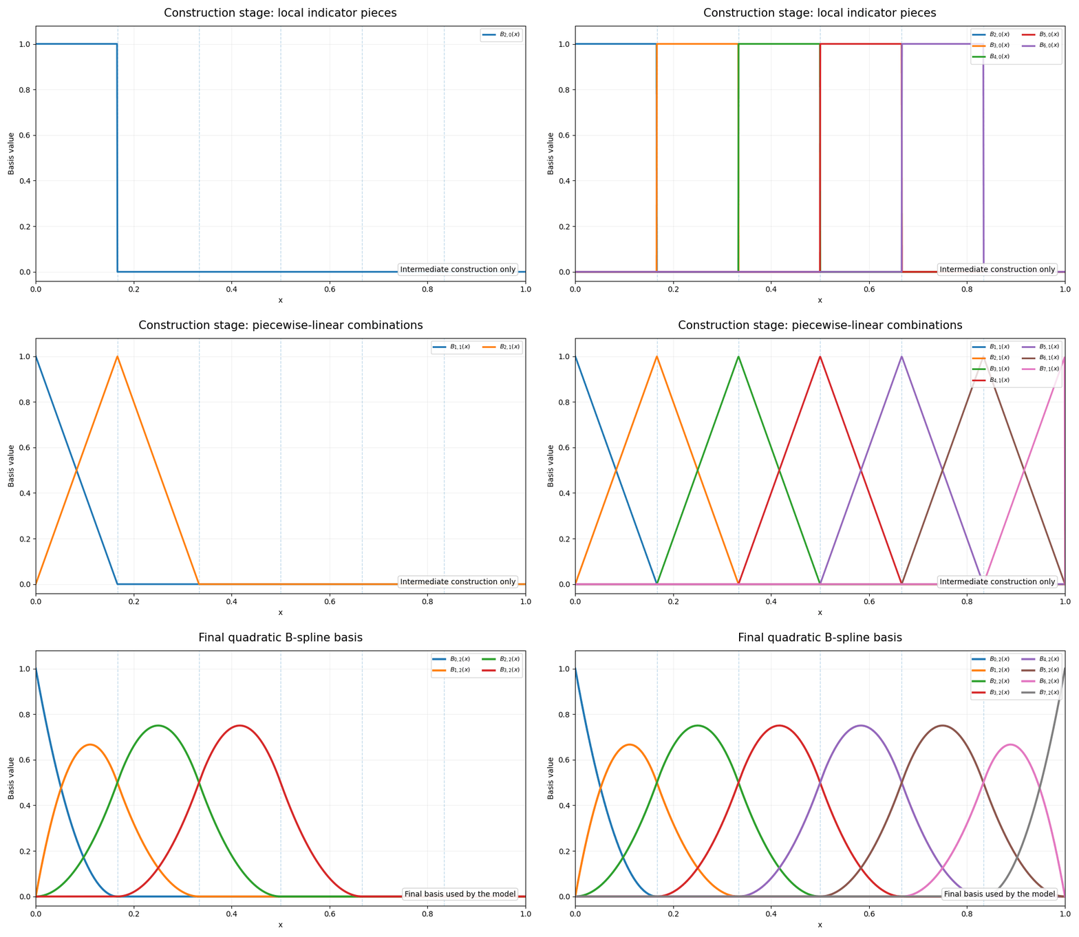
Unlike the powers used in a global polynomial, each quadratic B-spline basis function has local support,

Each coefficient therefore influences only a limited region of the fitted curve. With simple interior knots, the neighboring quadratic pieces also join with a continuous first derivative [7].

Once the basis functions are formed, the $i$-th observation is represented by

Stacking these rows gives the familiar regression model,

Polynomial and spline regression therefore differ in how $boldsymbol{Phi}$ is constructed, but both remain linear in the unknown coefficients once the basis is fixed.

With the representation problem in place, we can now return to the first question: which observations should the estimator trust?

Not All Bad Data Is the Same

When Measurements Are Missing

Measurements can go missing because of dropouts, failed recordings, or skipped readings. Missing values may be removed, imputed, or handled through probabilistic methods such as Expectation–Maximization [6]. Here, we deliberately use the simplest option—prefiltering measurements containing non-finite values—because our interest lies in the effect of outliers on curve fitting. This should not be interpreted as a general recommendation for handling missing observations.

valid = np.isfinite(Phi).all(axis=1) & np.isfinite(y)Phi = Phi[valid]y = y[valid]

Once the explicitly missing measurements have been handled, a more difficult problem remains: what should we do with observations that are present but unreliable?

The Outlier Problem

Outliers can appear because of faulty readings, interference, or unusual operating conditions. Unlike missing values, they are present and finite, and may initially look perfectly legitimate.

This creates a chicken-and-egg problem: we need a reliable model to determine which observations are inconsistent with the underlying relationship, but those same observations can distort the model used to identify them.

Robust estimators address this problem by limiting the influence of observations that are inconsistent with the fitted relationship.

The Same Six Estimators, a Different Basis

Changing the basis does not require us to redesign the robust estimator.

Huber regression reduces the influence of large residuals [1]. RANSAC searches for a consensus among the observations [2]. GNC-GM and GNC-TLS gradually transform easier optimization problems into more aggressive robust objectives [3]. ASOR adaptively estimates how strongly each observation should contribute to the fit [4].

For weighting-based robust estimators, the regression step can still be written as

What changes is the basis used to construct the feature vector.

For a cubic polynomial,

whereas for an eight-function spline,

The basis determines what shapes the model can represent. The robust estimator determines how much each observation is trusted.

If the same estimators can be used with different bases, the next question is whether they still behave the same way as the model becomes more flexible.

Stress-Testing

To answer that question, we repeat the same family of robustness experiments for curved models.

We consider three model classes,

and apply the same six estimators,

The benchmark covers several forms of contamination: zero-mean Gaussian replacement outliers, biased Gaussian replacement outliers, biased uniform replacement outliers, and observations generated from a coherent competing relationship. We also vary the contamination ratio from $0$ to $90$, the number of measurements, the nominal noise level, and record the computational cost. Each exact condition is repeated over 30 Monte Carlo realizations. The complete simulation notebook, full Monte Carlo results, and figures are available in the GitHub repository.

Prediction error is measured against the true noiseless relationship on a dense evaluation grid:

For the nominal-noise sweep, we also report

To isolate the effect of model richness from the effect of changing the underlying curve, we also perform a controlled experiment in which the same quadratic relationship and the same contaminated observations are fitted using all three bases. The models then use 3, 4, and 8 coefficients, respectively, while trying to recover exactly the same ground truth.

The interesting question is not simply whether robust estimation still works with curves, but what changes as the representation becomes richer.

Does estimator ranking change as the number of coefficients increases? How does RANSAC behave as its minimal sample grows? Do richer models require more data before their performance stabilizes? Does local spline support change how contamination deforms the fitted curve? And does computational cost change enough to alter the practical trade-offs?

What the Stress Tests Reveal

The controlled experiment gives the clearest view of what changes as the representation becomes richer. In each Monte Carlo realization, all three representations are fitted to the same $N=100$

At $30$ biased Gaussian contamination, GNC-TLS produces median NRMSE values of $0.246$, $0.276$and $0.485$ for the quadratic, cubic, and spline representations. ASOR follows a similar pattern, with of $0.257$, $0.307$and $0.469$. The move from three to four coefficients therefore causes only a modest loss. The eight-function spline is noticeably more demanding.

RANSAC reacts much more strongly. Under the same data and contamination level, its median NRMSE rises from $0.273$ for the quadratic fit to $0.383$ for the cubic and $1.384$ for the spline.

The effect is visible even without contamination: RANSAC’s median NRMSE increases from $0.179$ for the quadratic model to $0.625$ for the spline.

A richer basis can represent more shapes, but it also gives the estimator more parameters to recover.

RANSAC is particularly sensitive because its minimal sample grows with the number of coefficients.

For the three models considered here,

If the inlier fraction is $w$, the number of hypotheses needed to obtain an all-inlier minimal sample with confidence $p$ is

At $50$ contamination and $p=0.999$

The runtime results tell the same story. At $50$ biased Gaussian contamination, median RANSAC runtime increases from about $2.1$ms for the quadratic model to $3.4$ms for the cubic and $17.4$ms for the spline.

The algorithm itself has not changed. The model it must hypothesize has.

Richer Models Need More Data

The sample-size sweep shows the other side of the trade-off. Under $50$ biased Gaussian contamination, the spline becomes much more stable as more measurements are available.

For the spline, GNC-TLS NRMSE falls from $1.641$ at $N=50$

OLS behaves differently. Its error remains high even as the number of measurements grows, because additional data reduce variability but do not remove the systematic pull created by the contamination.

So the lesson is not that splines are inherently less robust.

Flexible models need enough trustworthy data to support the extra degrees of freedom.

The Contamination Pattern Still Matters

There is no universal estimator ranking.

Under biased contamination, GNC-TLS and ASOR generally provide the lowest prediction errors through moderate contamination, with GNC-GM often close behind.

When the replacement errors are zero mean, however, the differences become much smaller. For the spline at $50$ zero-mean Gaussian contamination, the median NRMSE values are $0.526$ for Huber, $0.540$ for GNC-GM, $0.554$ for ASOR, and $0.579$ for GNC-TLS.

In this benchmark, zero-mean replacement errors are generally less damaging than similarly scaled biased errors because they do not consistently push the fit in one direction.

The nominal-noise sweep gives another useful check. After normalizing by $sigma_{mathrm{in}}$

Local Support Contains Distortion; It Does Not Remove It

Splines introduce an effect that global polynomials do not have: local support.

In an illustrative experiment, we contaminate only part of the observations inside a narrow region while leaving the remaining local measurements nominal.

With OLS, the cubic polynomial gives an RMSE of about $22.6$ inside the contaminated region and $13.6$ outside it. The spline is distorted more strongly inside the contaminated region, with an RMSE of $40.9$, but slightly less outside it, at $12.1$.

This is an important distinction.

Local support can confine deformation to a smaller region, but it does not make contaminated observations harmless.

Once robust weighting is introduced, the distortion drops substantially for both representations. In this example, ASOR reduces the local and nonlocal errors to approximately $7.0$ and $4.8$ for the cubic model, and $12.6$ and $5.5$ for the spline.

The two mechanisms therefore solve different problems:

Local support controls where model flexibility acts. Robust estimation controls how strongly unreliable observations act.

When the Outliers Form Another Curve

Random replacement outliers are difficult, but a coherent competing relationship creates a different problem.

At low and moderate contamination, the robust estimators can still recover the nominal curve. As the two structures approach equal representation, however, the problem becomes ambiguous and different Monte Carlo realizations may favor different relationships.

Once the competing curve becomes the majority structure, the robust estimators generally follow it.

This is not simply an optimization failure. A single-model estimator has no way to know which of two internally consistent relationships is the physically correct one without additional information.

Robust estimation can suppress observations that disagree with the dominant model.

It cannot decide which of two coherent models should be trusted.

Taken together, these experiments show that changing the basis affects more than the shapes a model can represent. It also changes how much data the estimator needs, how expensive consensus-based methods become, and how contamination propagates across the fitted curve.

The controlled experiments isolate these effects. We now turn to application-inspired examples where robustness and model flexibility become separate practical requirements.

Case Study 1: Wind-Turbine Power Curves

Robustness is not the same as model flexibility.

Wind-turbine power curves describe the expected relationship between wind speed and generated power. Reliable estimation of this relationship is useful for performance monitoring and for identifying operating conditions that deviate from normal turbine behavior.

In practice, SCADA records may contain low-power or otherwise abnormal observations caused by curtailment, faults, shutdowns, or measurement issues [8]. These observations can distort the estimated nominal power curve, making this a natural application for robust regression.

The wind-turbine example is particularly useful because it separates two problems that are often confused:

Can the estimator resist abnormal observations?

and

Can the chosen model represent the underlying relationship?

To make this distinction clear, we first construct a region in which polynomial regression is the correct model. We then extend the domain until a single global polynomial becomes only an approximation.

First Isolate the Robustness Problem

For this synthetic example, let the rated speed be $12,text{m/s}$.

Below rated speed, define

and

Because $t$ is linear in $v$, this expression is exactly a cubic polynomial in wind speed.

If we fit a cubic polynomial over this region, the model family is correctly specified. The experiment therefore isolates the effect of contamination.

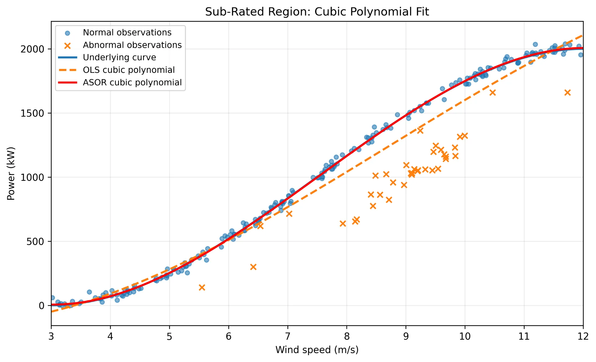
For this realization, the prediction RMSE is approximately $91.4,text{kW}$ for OLS and $2.7,text{kW}$ for ASOR.

Here the interpretation is straightforward:

The model was appropriate. The estimator was the problem.

Robust estimation addresses the contamination problem without requiring us to change the model family.

Then Expose the Representation Problem

Now extend the same ground truth beyond rated speed:

The relationship is now piecewise defined:

One global polynomial is no longer the true model.

No nonconstant finite-degree polynomial can exactly reproduce this shape. If a polynomial $q(v)$ satisfies $q(v)=2000$

A global polynomial can therefore only approximate the curved-to-flat relationship.

The problem has changed. We are no longer asking only whether the estimator is robust; we must also ask whether the chosen basis can represent the underlying relationship.

Can a Higher-Order Polynomial Solve the Problem?

One obvious response is to increase the polynomial degree.

A fourth-order polynomial uses

This provides more flexibility than a cubic, and with robust estimation it performs reasonably well.

However, all five polynomial basis functions remain global. The same coefficients must simultaneously describe the low-speed rise, the steep middle region, the transition near rated speed, and the high-speed plateau.

A spline adds flexibility differently. Instead of introducing increasingly high global powers, it uses locally supported basis functions that can adapt to different parts of the curve.

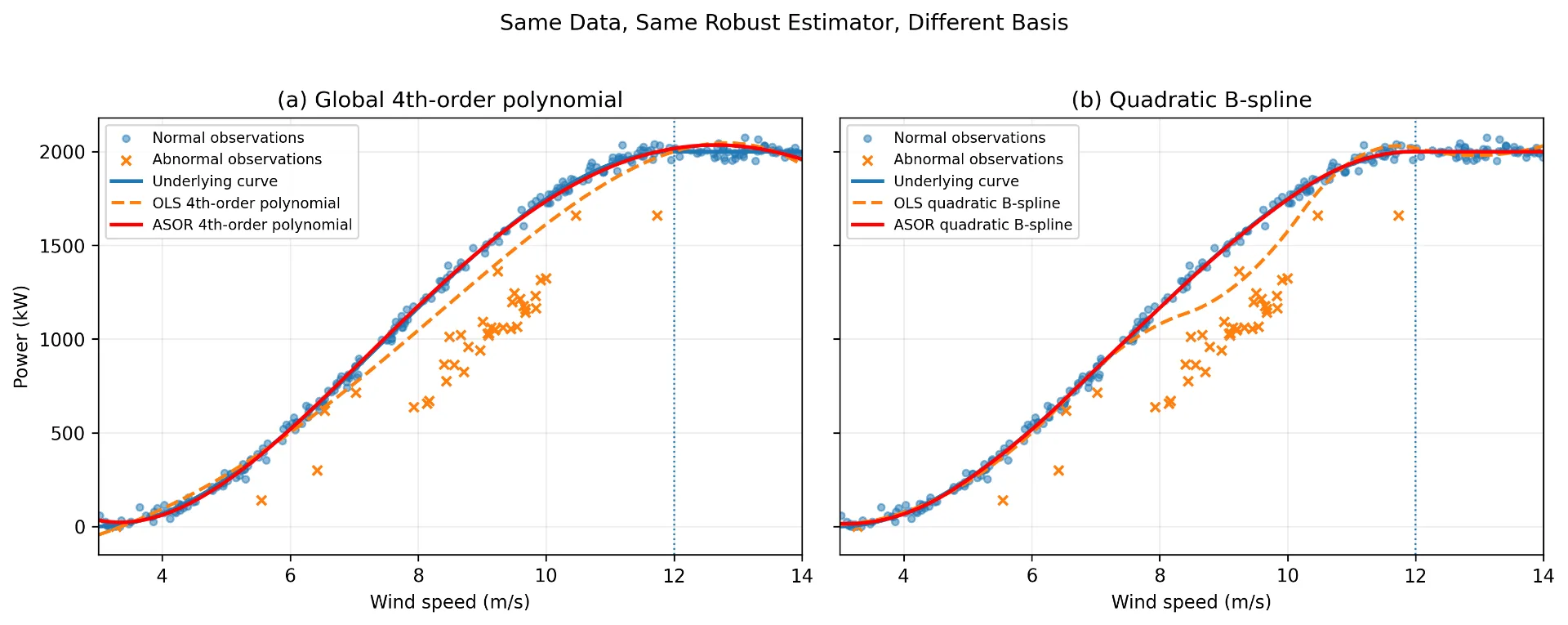
For the same illustrative realization, over the full $3–14,text{m/s}$ interval, the ASOR fourth-order polynomial gives an RMSE of approximately $14.5,text{kW}$, compared with $4.2,text{kW}$ for the ASOR quadratic B-spline.

That distinction is important:

Robust estimation can stop abnormal observations from bending a good model. It cannot turn the wrong basis into the right one.

In this example, ASOR addresses the contamination, while the spline addresses the representation.

Case Study 2: Predicting Where GNSS Doppler Goes Next

GNSS Doppler evolves smoothly with satellite–receiver motion. Short-term prediction can help bridge brief measurement gaps and provide an expected Doppler trend against which abnormal measurements associated with interference or tracking disturbances can be compared.

This makes Doppler prediction a useful robust-regression example: corrupted measurements can distort the fitted trend and, consequently, the predicted Doppler.

Over a short observation window, we use a low-order polynomial as a compact local approximation to the Doppler trajectory.

The workflow is

The example contains both missing and corrupted measurements. Missing samples are excluded according to the preprocessing assumption introduced earlier, while corrupted samples remain in the data and must be handled by the estimator.

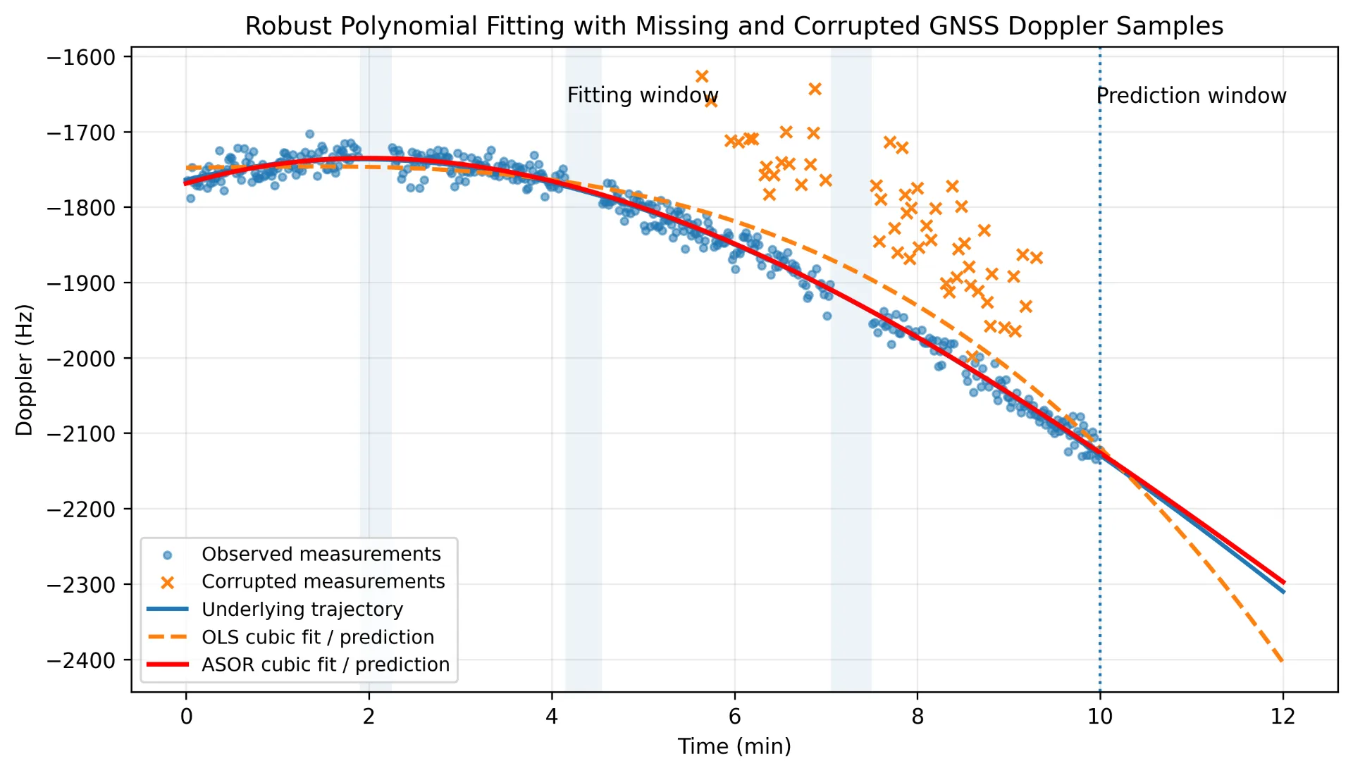
OLS tries to explain the corrupted measurements, causing the fitted polynomial to bend toward the corrupted cluster. ASOR reduces their influence and preserves a trajectory that remains much closer to the nominal Doppler evolution.

This becomes particularly important when the fitted curve is extrapolated beyond the observation window. A moderate fitting error inside the observed region can grow substantially when the polynomial is projected into the future.

In this synthetic illustration, the short-horizon prediction RMSE is approximately $46.4,text{Hz}$ for OLS and $7.9,text{Hz}$ for ASOR.

The claim here is deliberately local. A satellite Doppler trajectory is not assumed to follow one cubic polynomial indefinitely. Instead, a low-order polynomial provides a compact approximation over a short observation window.

This leads to another important lesson:

Interpolation and extrapolation are not the same problem.

Robust fitting can improve both, but extrapolation remains inherently more sensitive because future points are no longer surrounded by observed data.

What Survives When the Line Becomes a Curve?

The most useful lesson from all of these examples is not tied to one polynomial degree or one particular spline.

It is the basis view.

A straight line uses

A polynomial uses

A spline replaces global powers with locally supported functions,

Once the basis is fixed, all of these models return to the same form:

That is why the robust estimators transfer so naturally.

The practical workflow is therefore straightforward:

1. Choose a basis that can represent the relationship of interest.

2. Center and scale predictors when polynomial powers become poorly conditioned.

3. Remove identifiable missing rows before fitting when complete-case analysis is appropriate.

4. Use robust estimation when finite observations may still be contaminated.

5. Use enough observations to support the chosen basis.

6. Treat extrapolation more cautiously than interpolation.

A richer basis makes the model more expressive, but it does not make unreliable observations trustworthy. Robust estimation makes the fit less sensitive to contamination, but it cannot rescue an inappropriate model.

Those are two different problems.

Next in the series. We move beyond polynomials and splines to richer representations for capturing complex nonlinear and periodic structure.

References

[1] P. J. Huber, “Robust Estimation of a Location Parameter,” The Annals of Mathematical Statistics, vol. 35, no. 1, pp. 73–101, 1964.

[2] M. A. Fischler and R. C. Bolles, “Random Sample Consensus: A Paradigm for Model Fitting with Applications to Image Analysis and Automated Cartography,” Communications of the ACM, vol. 24, no. 6, pp. 381–395, 1981.

[3] H. Yang, P. Antonante, V. Tzoumas, and L. Carlone, “Graduated Non-Convexity for Robust Spatial Perception: From Non-Minimal Solvers to Global Outlier Rejection,” IEEE Robotics and Automation Letters, vol. 5, no. 2, pp. 1127–1134, 2020.

[4] A. H. Chughtai, M. Tahir, and M. Uppal, “Bayesian Heuristics for Robust Spatial Perception,” IEEE Transactions on Instrumentation and Measurement, vol. 73, pp. 1–11, 2024.

[5] T. Hastie, R. Tibshirani, and J. Friedman, The Elements of Statistical Learning: Data Mining, Inference, and Prediction, 2nd ed., Springer, 2009.

[6] R. J. A. Little and D. B. Rubin, Statistical Analysis with Missing Data, 3rd ed., Wiley, 2019.

[7] C. de Boor, A Practical Guide to Splines, revised ed., Springer, 2001.

[8] Y. Wang, D. G. Infield, B. Stephen, and S. J. Galloway, “Copula-Based Model for Wind Turbine Power Curve Outlier Rejection,” Wind Energy, vol. 17, no. 11, pp. 1677–1688, 2014.

Get in touch 👋

For more of my work, explore my GitHub, or connect with me on LinkedIn. I welcome questions, new ideas, and opportunities to collaborate in Data science, AI and Statistical Signal Processing. If you enjoy my articles, sharing them with others helps these conversations reach more people.

All data-driven figures were generated via simulations by the author. The featured image was created with the assistance of AI.