
Consider a situation where a plan must be made to satisfy demand 95% of the time. A 0.95 expectile may seem like the right answer; however, the level of the expectile does not represent the proportion of values below the expectile.
A variable uniformly distributed between 0 and 1 has a 95th percentile equal to 0.95. The 0.95 expectile of that variable is approximately 0.8134. Therefore, only 81.34% of the distribution lies below 0.8134.
A quantile defines a decision boundary, and an expectile is set to minimize the asymmetric squared error. We will compute the asymmetric losses and compare decisions using the two loss functions in Python. Synthetic data will be used for all examples.
Contents
- Start with the question the statistic answers
- Change the power, change the target
- An exact counterexample: uniform data
- Compute both statistics in Python
- Keep the ranks. Move one observation.
- Choose the statistic by the cost of being wrong
- Three checks before using the result
- The distinction to carry into practice
- How the examples were checked
- References
Start with the question the statistic answers
A cumulative distribution function gives the probability that a random variable is less than or equal to a given value. For a continuous, strictly increasing CDF, the value associated with a cumulative probability of alpha gives us the quantile at level alpha. More generally, the coverage of a quantile is given by:
A distinction needs to be made for tied observations. A jump in the cumulative distribution may cross the requested level. Thus, for a sample quantile, the proportion of the sample at or below its quantile need not equal alpha exactly. A percentile is a special case of a quantile, where the level is expressed in terms of 100. [4]
Expectiles rely on distances from a reference value. Values above the reference pull it up, and values below pull it down. The asymmetry parameter determines the relative pulling strength, and the distance of the observation determines how strongly it pulls.
We will consider some special cases to begin. The 0.5 expectile is the mean. The median is the 0.5 quantile. [2, 3]
Change the power, change the target
A residual is the difference between an observed value y and a given decision value t. A positive residual indicates the decision was less than the value. Using alpha between 0 and 1, positive residuals are given weight alpha, and negative residuals are given weight 1 – alpha.
When the expected absolute error is finite, quantiles are determined by minimizing expected absolute errors weighted asymmetrically (pinball loss). For a sample, the expectation is replaced by the average loss. [1]
Expectiles are similar to quantiles, and both rely on asymmetric weighting. However, expectiles are based on squared errors. Therefore, the effect of an observation on the expectile value depends on how far the observation is from the expectile. [2]
With an alpha of 0.95, the weights are 0.95 and 0.05: a 19-to-1 ratio. Both objectives penalize underestimation more heavily. Under absolute loss, doubling an error doubles its contribution on that side. Under squared loss, doubling it multiplies the contribution by four. The same weights can therefore lead to different optimal decisions.
An exact counterexample: uniform data
Let Y be uniform on [0, 1]. Its cumulative distribution function (CDF) is given by y for y ∈ [0, 1], and consequently, its 95th percentile is 0.95. We will calculate its expectile directly.
At the expectile, the derivative of expected asymmetric squared loss is zero. The weighted expected distances on either side of the decision are equal [3]:
Expectiles rely on the magnitude of the outcomes as well as the frequency. For a candidate expectile e in [0, 1] and a uniform random variable Y in the interval [0, 1], these expectations may be written as:
Substituting the above in the balance equation and taking the positive square root completes the calculation.
For example, when α = 0.95, expectile = 0.8133945. Coverage below this expectile is approximately 81.34%. Coverage below the 95th percentile is 95%, which is 13.66 percentage points greater than expectile coverage.
Expectiles are distribution dependent and therefore a calculation of this form does not represent a general conversion of an expectile to a percentile.
Compute both statistics in Python
SciPy calculates expectiles. The example uses NumPy’s inverted-CDF method to evaluate sample quantiles. NumPy has other sample-quantile methods; the default is linear interpolation. Specifying this method is needed for clarity. [3, 4]
The sample has a value of 100 and 99 values of 0. The 95th percentile of the sample is 0, and the 0.95 expectile is approximately 16.10. The value of 100 pulls the expectile above the percentile.
In this example, 99% of the observations are less than or equal to both the quantile and expectile. In the current situation, the cumulative distribution function (cdf) jumps from 0 to 0.99 at the value 0. This defines the 0.95 quantile.
Keep the ranks. Move one observation.
99 zeros and a single value M > 0 define the sample. The 0.95 quantile remains at 0, regardless of the magnitude of M. The proportion of positive values is unchanged.
The expectile is linearly related to M and is greater than the quantile, which is fixed in this case.
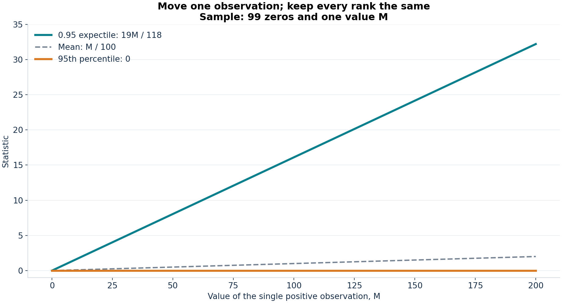
When M is 10, the expectile is approximately 1.6102. When M is 100, the expectile is approximately 16.1017. Both of these cases have a 95th percentile of 0. Of course, this creates a problem if a large positive observation is recorded due to a mistake.
Before taking any action based on the expectile, determine whether the large observation represents a valid case or is an error in data entry. The expectile is affected by both cases.
Choose the statistic by the cost of being wrong
This example considers an illustrative planning case where demand is assumed to be uniformly distributed between 0 and 100. In the first case, the cost of underestimating demand by one unit is 19 times the cost of overestimating demand by one unit. This is known as asymmetric absolute loss. In the second example, the costs also vary with a 19 to 1 weight, but are based on the squared value of the error.
The first goal is to reach a 0.95 quantile. The second is to reach a 0.95 expectile. For this case, the true (population) values for decisions are 95 units and 81.34 units, respectively. We change the target by altering the cost curve, but the asymmetry ratio is the same.
The experiment uses 100 independent runs. Each run generates a training set of 400 samples and a test set of 10,000 samples. From the training set, it determines the mean, the 0.95 quantile and the 0.95 expectile. It evaluates each of these three decisions on the test set. The random number generator seed is set to 20261031. All decisions are evaluated on the same set of samples for a given case.
Losses will be determined using the weights 0.95 and 0.05, equivalent to dividing penalties of 19 and 1 by 20. Absolute loss will be expressed in demand units and squared loss will be expressed in demand units squared. Expectile and quantile decisions are compared within each loss function.
Table 1. Average decisions and test results across 100 synthetic repetitions.
|
Decision |
Estimated value |
Test coverage |
Asymmetric absolute loss |
Asymmetric squared loss |
|---|---|---|---|---|
|
Mean |
50.02 |
49.95% |
12.53 |
418.53 |
|
Quantile |
94.73 |
94.72% |
2.38 |
142.14 |
|
Expectile |
81.33 |
81.25% |
3.32 |
110.63 |
On average, the estimated 0.95 quantile and expectile were 94.73 and 81.33, respectively. The average coverage of the 0.95 quantile and expectile was 94.72% and 81.25%, respectively. These small deviations from the true population values are due to limited training observations and variation in the test observations.
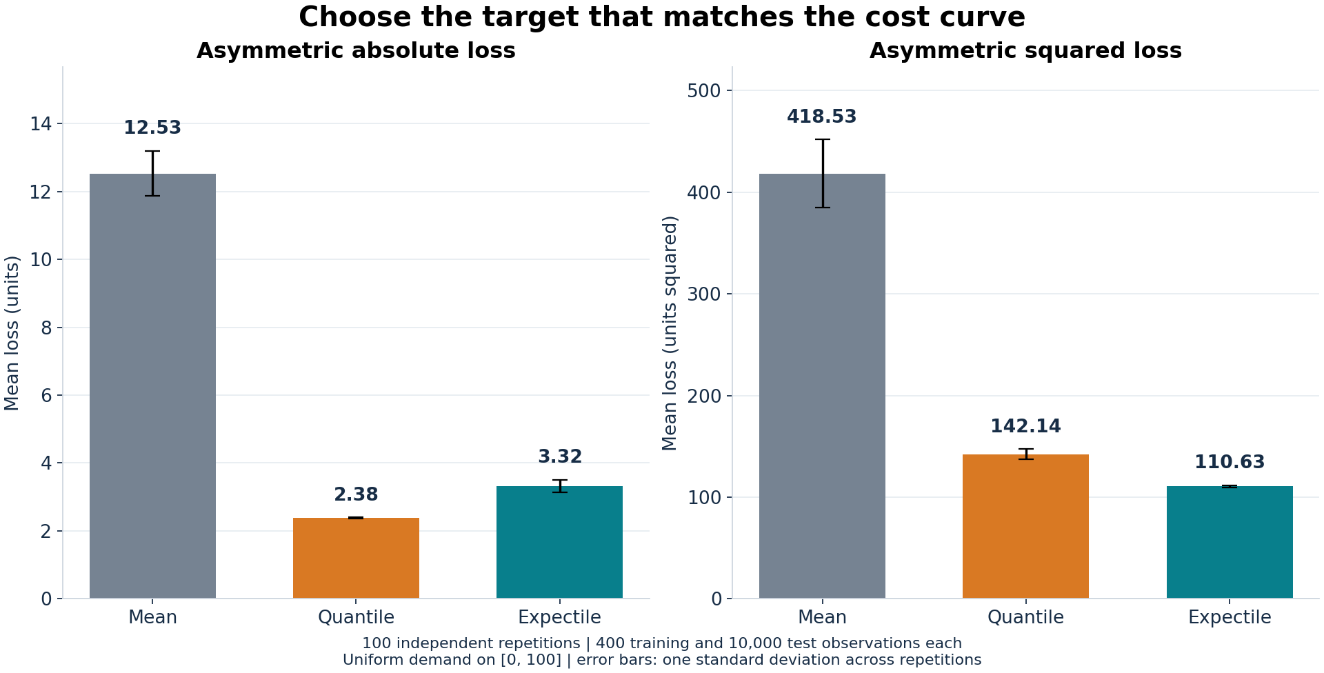
Over the 100 simulations, the average asymmetric absolute test loss for the expectile was 3.32, compared to 2.38 for the quantile. The average asymmetric squared test loss incurred by the expectile was 110.63 and by the quantile was 142.14.
Since the absolute and squared losses are expressed in different units, we cannot determine the best decision based on loss magnitude. For the case at hand, evaluate the decisions using the cost function pertinent to the situation.
Three checks before using the result
Let us first write down the requirement and then choose a corresponding statistic. Assume the demand is continuous. For a coverage level of 0.95, we look to the 0.95 quantile. The 0.95 expectile answers a weighted squared-loss question. We should keep in mind that we cannot be certain about the future performance of the estimator.
Second, the quality of data and the nature of the population should be evaluated. The ordinary population squared-loss formulation assumes a finite second moment. A finite sample can still return a number when its population counterpart has problematic moments, and a small number of very large observations can strongly influence an estimate. More advanced expectile formulations require their own assumptions.
Third, understand the difference between a distribution summary and a forecasting model. Here, decisions are constant, and observations are synthetic and independent. A conditional expectile model would estimate a target given features, and a forecasting application would need an evaluation design that reflects when information becomes available. This example does not create a conditional expectile or a forecasting model.
The distinction to carry into practice
Prior to setting an upper limit, determine the nature of the claim to be evaluated. A coverage target requires determination of the relevant quantile and an assessment of the estimated coverage. On the other hand, an asymmetric squared error function requires determination of the expectile and choice of weights based on the cost function. In the example with a uniform distribution, a level of 0.95 represents 95% coverage for the quantile, but only 81.34% for the expectile. The level must be assessed in the context of the question being answered.
How the examples were checked
The analysis script, executed on Python 3.9.6, NumPy 2.0.2, SciPy 1.13.1 and Matplotlib 3.9.4, generated all results presented. Results were validated using analytical examples. Expectiles were also calculated using a partitioning method and compared to solutions from direct numerical optimization of the squared-loss function.
References
[1] R. Koenker and G. Bassett Jr., Regression Quantiles (1978), Econometrica 46(1), 33–50.
[3] SciPy contributors, scipy.stats.expectile (accessed 31 October 2026), SciPy 1.13.1 documentation.
[4] NumPy contributors, numpy.quantile (accessed 31 October 2026), NumPy 2.0 documentation.